Empirical Data Analysis
A New Tool for Data Analytics
Plamen Angelov, Fellow, IEEE,Xiaowei Gu, and Dmitry Kangin Data Science Group,
School of Computing and Communications, Lancaster University, Lancaster, UK
E-mail: [email protected]
Jose Principe, Fellow, IEEE Computational Neuro Engineering Laboratory,
Department of Electrical and Computer Engineering, University of Florida, Grainsville, FL, USA,
E-mail: [email protected]
Abstract—In this paper, a novel empirical data analysis approach (abbreviated as EDA) is introduced which is entirely data-driven and free from restricting assumptions and pre-defined problem- or user-specific parameters and thresholds. It is well known that the traditional probability theory is restricted by strong prior assumptions which are often impractical and do not hold in real problems. Machine learning methods, on the other hand, are closer to the real problems but they usually rely on problem- or user-specific parameters or thresholds making it rather art than science. In this paper we introduce a theoretically sound yet practically unrestricted and widely applicable approach that is based on the density in the data space. Since the data may have exactly the same value multiple times we distinguish between the data points and unique locations in the data space. The number of data points, k is larger or equal to the number of unique locations, l and at least one data point occupies each unique location. The number of different data points that have exactly the same location in the data space (equal value), f
can be seen as frequency. Through the combination of the spatial density and the frequency of occurrence of discrete data points, a new concept called multimodal typicality, τMM is proposed in this paper. It offers a closed analytical form that represents ensemble properties derived entirely from the empirical observations of data. Moreover, it is very close (yet different) from the histograms, from the probability density function (pdf) as well as from fuzzy set membership functions. Remarkably, there is no need to perform complicated pre-processing like clustering to get the multimodal representation. Moreover, the closed form for the case of Euclidean, Mahalanobis type of distance as well as some other forms (e.g. cosine-based dissimilarity) can be expressed recursively making it applicable to data streams and online algorithms. Inference/estimation of the typicality of data points that were not present in the data so far can be made. This new concept allows to rethink the very foundations of statistical and machine learning as well as to develop a series of anomaly detection, clustering, classification, prediction, control and other algorithms.
Keywords—empirical data analysis; multimodal typicality; data-driven; recursive calculation; inference; estimation.
I. INTRODUCTION
Most of the human activities have already been largely changed in the recent decades because of the very fast development of information technologies and the Internet. Astronomical and ever increasing amount of data is being generated every day. As a result, data analysis is a rapidly growing field due to the strong need of processing large data
sets or streams and converting the data into useful information.
Traditional approaches are based on a number of restrictive assumptions which usually do not hold in reality. This applies to the fuzzy sets theory [1] with its subjective way of defining membership functions, assumption of smooth and pre-defined membership functions. It also applies to the probability theory [2] and statistical learning [3], [10]. They are an essential and widely used tool for quantitative analysis of data representation of stochastic type of uncertainties. However, they rely on a number of strong assumptions including pre-defined smooth and “convenient to use” types of probability distribution, infinite amount of observations/data points, independence between data points (so called iid – independent and identically distributed data), etc. However, in most practical problems, these assumptions are not satisfied. Till now, several alternative methods [5], [6] have been proposed aiming to avoid the problem of unrealistic prior-assumptions and get closer to the data rather than stick to the theoretical prior assumptions, but these methods still use at some point assumption of (albeit local) Gaussian/normal distribution.
In this paper, we introduce a novel empirical data analysis (EDA) approach. It is a further development of the recently introduced TEDA (typicality and eccentricity data analytics) framework [7]-[9]. It does not require any prior assumptions which are usually unrealistic and restrictive, or parameters. Instead, it is entirely based on the empirical observations of discrete data points and their mutual position forming a unique pattern in the data space. It starts with calculating (recursively) the cumulative proximity, ; then the standardized eccentricity, ; and the density, D and finally, the multimodal typicality, MM. Moreover, unlike the pdf where identifying the
number and position of modes is a well known problem usually solved by clustering, the multimodal typicality, MM is
derived from the data automatically and without clustering or other additional algorithm. It is often quite close to the histograms but is not the same since it does take into account the mutual position of the data as well as the frequency of their occurrence, f.
The advantages of multimodal typicality, MM are obvious
because it combines pdf, histogram and mutual distributions of the data points together and has a closed analytical form that can be manipulated further. In addition, multimodal typicality,
MM can be calculated recursively, which makes it suitable for
applications to online data streams.
Moreover, one can infer the typicality , (x) for any feasible value x by interpolation or extrapolation and the typicality can be used in a manner similar to probability because it has same properties of being between 0 and 1 and summing up to 1. It is demonstrated in this paper that it can be used to build a naïve typicality-based EDA Classifier [10] which not only provides better results than the naïve Bayes classifier (due to taking into account the actual distribution of the data) but also in comparison with the SVM classifier [11]. In addition to that, the naïve EDA Classifier does not require any prior assumption of the distribution of the data selection of the type of the kernel or threshold constants or iterative optimization as the SVM approach does.
Another very interesting feature is that this new method is free from some paradoxes that the traditional probability density function has [12]. Additionally, it combines effectively the two different types of randomness representation: a) the one based on the ratio of number of times a discrete random variable occurs (
k k
pklim *; where k* is the number of times of occurrence and k is the total number of data points/observations), see Fig.2 and b) the one based on pdf, see Fig.1(d). In the probability theory and statistics literature the transition between a) and b) is often neglected. In fact, a) (the multuimodal version, MM) is suitable for games such as
dices, coins, balls etc. or “pure” random processes, white noise type while b) (the unimodal typicality, τ) is applicable to most of the real processes which are a more complex mixture of deterministic and random or, more correctly, complex phenomena. The proposed typicality works well for both a) and b) and combines them in a unique closed form representation without assuming k a type of the distribution, or any user- or problem- specific parameters.
This novel non-parametric and assumption-free empirical data analysis framework is very promising and attractive because it is entirely based on the actual discrete/digital data and we live in the era of big (digital) data revolution. It is logical to develop and use methodologies and approaches that are suitable and tailored to this reality rather than stick to methods that were introduced centuries ago analyzing primarily analog signals and pure random phenomena like games or assume distributions a priori.
The rest of this paper is organized as follows: section II introduces the novel empirical data analysis (EDA) framework including the theoretical basis, multimodal typicality and the recursive calculations. Section III describes the method of making inference within this novel framework. An additional example of multimodal typicality and inference of a benchmark dataset is presented in section IV. The naïve EDA Classifier is introduced and results of its application to benchmark problems compared with other classifiers in section V. Finally, the conclusions and future directions are provided in section VI.
II. EMPIRICAL DATA ANALYSIS FRAMEWORK
First, let us introduce the main quantities that represent ensemble properties of the data within EDA:
1) cumulative proximity,
2) standardized eccentricity,
3) density, D, and finally 4) typicality, .
In addition, the calculations can be recursive and the multimodal form of the typicality is also introduced.
A. Theoretical Basis
First of all, let us consider the real Hilbert spaceRdand
assume a particular data set or stream denoted as
dk R x x
x1, 2,..., , where the subscripts denote the time instance at which the data point arrives. Within the data set/stream, some of the data points may repeat more than once, namely,i,jxixj. The set of unique data point locations at
time instance k can be defined as
d l R u uu1, 2,..., and the corresponding number of times
f1,f2,...,fl
different datapoints occupy the same unique locations ( fi can be viewed as
frequency if it is divided by k). Obviously, always
l
k
, but more often in real problems because of having exactly the same values many times,l
k
. Based on
u1,u2,...,ul
and
f1,f2,...,fl
, we can reconstruct the data set
x1,x2,...,xk
exactly if needed regardless of the order of arrival of the data points. Further in this paper, all derivations are conducted at the kth time instance by default if there is nospecial declaration.
1) Cumulative proximity
Cumulative proximity is a measure indicating the degree of closeness/similarity of a particular data point to all other existing data points [7]-[9].
The cumulative proximity of the unique data point ui is
expressed as follows:
l d
i lj i j i
u
k , , ,12,...,
1
2
u u u
(1)
where d
ui,uj is the distance between two unique locations iu and uj. The distance can be of Euclidean, Mahalanobis
type, based on cosine [12] any other metric.
2) Standardized eccentricity
Eccentricity was introduced in [7]-[9] to represent the association of the data point with the tail of the distribution and the property of being an outlier/anomaly [8]. The standardized eccentricity of ui(i ,12,...,l) is calculated as
follows:
2
,E
0,k ,1l1E u ku
k i u k i u
k u
u u
u
(2)
where,i ,12,...,l,
l
j j
u k u
k l
E
1
1 u
u
.
It is interesting to note that l
li i u
k 2
1
u .
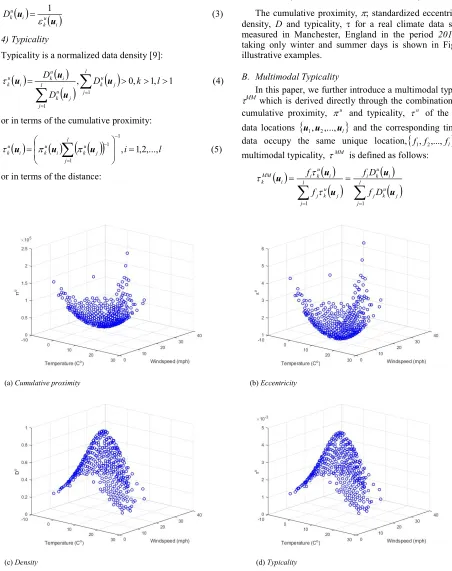
(a) Cumulative proximity (b) Eccentricity
[image:3.612.73.525.89.660.2]
(c) Density (d) Typicality
Fig. 1. The cumulative proximity, standardized eccentricity, density and typicality of the unique data points of climate dataset
Data density is inversely proportional to the standardized eccentricity [9]. The density of ui(i ,12,...,l) is defined as
follows:
i u k i u k
D
u u
1
(3)
4) Typicality
Typicality is a normalized data density [9]:
, 1
0, ,1 1 1
l k D
D
D l
j j
u k l
j j
u k i u k i u
k u
u u u
(4)
or in terms of the cumulative proximity:
l
i lj j
u k i u k i u
k , ,12,...,
1
1
1
uu
u
(5)
or in terms of the distance:
1
1
1
1 2
1
2 , ,
lv l
j v j
l
j i j
i u
k u d u u d u u
(6)
The cumulative proximity, ; standardized eccentricity, ; density, D and typicality, for a real climate data set [13] measured in Manchester, England in the period 2010-2015
taking only winter and summer days is shown in Fig. 1 as illustrative examples.
B. Multimodal Typicality
In this paper, we further introduce a multimodal typicality,
MMwhich is derived directly through the combination of the
cumulative proximity, u and typicality, u of the unique
data locations
u1,u2,...,ul
and the corresponding times thedata occupy the same unique location,
f1,f2,...,fl
. Themultimodal typicality, MM is defined as follows:
l
j j
u k j
i u k i l
j j
u k j
i u k i i MM k
D f D f f
f
1 1
u u u
u u
Fig.2. A simple example of multimodal typicality
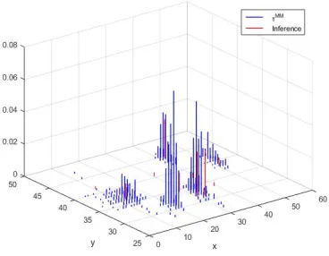
Fig.3. 3-dimensional multimodal typicality of the climate dataset
where
0,
0, ,1 11 1
f l f D k lj j
u k j l
j j
u k
j u u
A simple example to illustrate how multimodal typicality works for small values of k (amounts of data points) and the fact that it coincides with the frequency-based probability,
k k
pklim *[2],[4],[10] is shown in Figure 2 where a small data set of 3 data points is considered in which two of them have exactly the same value: x={2;5;5}. Obviously, u={2;5}; l=2; k=3; l<k. Naturally, the value of , MM={1/3;2/3} while for such small number of k it is not possible to get a meaningful pdf, but if follow the purely frequentistic form
k k
pklim * [2] the result will be exactly the same. Yet, the typicality (defined in equations (5)-(6)) automatically starts to approximate the pdf (see Figure 1(d)) for larger number of points and if use multimodal typicality (equation (7), which also takes into account the frequency, f) it provides a multimodal likelihood quite close to the histogram, see Figures 3-5.
To further investigate the advantages of the multimodal typicality, the 3-dimensional multimodal typicality,MM of the
climate dataset [13] is shown in Fig. 3. A comparison of MM
with the traditional histogram [4], [10] as well as with the normal (Gaussian) pdf [4], [10] is also made in a 2-D graph for visual clarity, shown in Figure 4.
The advantages of the multimodal typicality, MMcan be
summarized as follows:
1. This typicality takes the spatial density, D into consideration.
2. The frequency of the occurrence, f of a certain data sample is also taken into account.
3. There is no need for clustering algorithm, thresholds or any parameters or complicated pre-processing technology involved to generate the multimodal typicality distribution.
4. It provides in a closed analytical form without any prior
assumptions made.
Multimodal typicality, MM is a function having the
following properties: a) it sums up to 1;
b) it is very close to (but not the same as) the histogram; c) its value is within the range [0;1];
d) it combines the two completely different forms used so far: histogram and pdf in one expression;
e) it combines the two representations of the probability (frequency-based and distribution-based)
f) it is free from the paradoxes that pdf is related to [12]. For small values of k, the multimodal typicality is exactly the same as the frequentistic form of probability (see Fig. 2), and with large k, it tends to the pdf. For lkor lk(when there are different data points with the same value) different modes will appear automatically while for cases when lk
or lk one may still need clustering to get a multi-modal representation [12].
C. Recursive Calculations
Recursive calculations play a very significant role in online data streams processing [14]. With the utilization of recursive calculation, there is no need to keep large amount of data samples in the memory, which is more computation and memory efficient. The multimodal typicality, MMcan be
updated recursively as follows.
If the data point that arrives at time instance k+1, xk+1 is
not unique (there is already a point with exactly the same value), then the multimodal typicality can be updated as follows:
1
1
1 1
1
1 1
,
k i
i u k l
j j
u k j
i u k i
k j k i
i u k l
j j
u k j
i u k i
i MM k
D D f
D f
D D f
D f
x u u u
u
x u x u u u
u
u
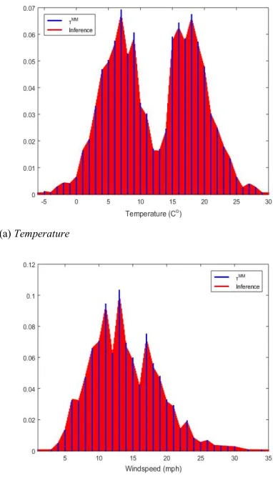
(a) Temperature
(b) Wind speed
Fig.4. Comparison of the multimodal typicality, histogram and Gaussian pdf of the climate dataset in 2-D
(a) Interpolation
(b) Extrapolation
(c) 3D multimodal typicality with inferences of 5 arbitrary data points
Fig.5. Examples of inference of multimodal typicality
In case, when the new coming data point, xk+1 has unique
new location,
u
l1 then the set of unique locations
u1,u2,...,ul
is being appended by ul1xk1 becoming
u1,u2,...,ul,ul1
and
f1,f2,...,fl
is also appendedbyfl11becoming
f1,f2,...,fl,fl1
or
f
1,
f
2,...,
f
l1,
.The cumulative proximity can be updated as follows:
i ku
i d i l
i lu
k1u u 2 u,u1, ,12,...
(9)
For the case when Euclidean distance is considered it becomes [7]-[9]:
1 1
1 1 1
T 1 1 1
1 1
l l l l l l lT l
u
k u l u u U
(10)
where l1ll1l l11ul1, (11)
1 T
1
1 1 11
l l l
l ll U l
U u u . (12)
After updating of the cumulative proximities, the typicality of all the unique data points including the new one at time
instance k+1 can be updated using (6) as well as their corresponding multimodal typicality at time instance k+1 can be updatedusing equation (7).
III. INFERENCE USING THE MULTIMODAL TYPICALITY
(a) Temperature
(b) Wind speed
Fig.6. Curves of empirical likelihood of the climate dataset in 2-D
proposed empirical data analysis framework, EDA will be introduced. The inference only applies to feasible points and therefore, first step is to check if a data point is feasible or not which is problem dependent, e.g. there cannot be a negative mass, distance, age, etc. For feasible values, we can then estimate the typicality as follows.
For the data sample that occupies a new unseen location, the set of unique locations is first updated by appending ul+1:
u1,u2,...,ul,ul1
. Then l1 and Ul1 are recursively updated using equations (11) and (12), and then, most importantly, calculate ku
ul1 using equations (6)-(10).If the data point at which an estimate/inference of the typicality is made is within the range of the dataset (that is, perform an interpolation, see Fig. 5(a), the red line) then the frequency fl1 is estimated as the average of the frequencies of the two nearest data points of each dimension:
d
i Ri Li
i L i l i R i R i L i l
l d u u uf uu u f
f
1 , ,
, ,1 , , , ,1
1 1 (13)
where uR,i and uL,i are the ith dimensional values of uR,iand i L,
u that are the nearest to ul1in the ith dimension and satisfy
i R i l i
L u u
u , 1, ,.
If the data point is outside of the range (that is, extrapolation, see Figure 5(b), the red line), the frequency is set to 1: fl11. Because such points for which inference is made do not actually exist (they are virtual), they should not influence the typicality of the other really existing data points. The density of the virtual data point is:
l
j l j
l
i l
j i j
l u k u k l
u k
d d l
E D
1 1
2 1 1
2
1 1
, 2
, 1
2 u u
u u
uu
u
(14)
Therefore, using equation (7) the typicality of any new data point can easily be estimated using Dku
ul1 and fl1:
l
j j
u k j
l u k l l MM k
D f D f
1 1 1 1
u u u
(15)
Fig. 5(c) depicts a 3D example with five feasible points for which an inference is made shown in red. In Fig. 6 inference for many points is made (in red) which leads to a typicality graph that looks like continuous (it is not continuous because the number of actual data points, k plus the points for which the inference is made is not infinite).
IV. EXAMPLE
In this section, another example of multimodal typicality,
MM and inference for a benchmark dataset is presented. The
benchmark dataset in question is a wrist-worn accelerometer (3 dimensional) data set for activities of daily life (ADL) recognition described in [15]. In this paper, only part of the data is used (5 clusters with 150 data points per cluster). The data is real and interesting because they are clearly not uni-modal. The proposed multimodal typicality can be determined without any clustering. It is visually very similar to the histograms that can be obtained. The 3D graph of the multimodal typicalityand inference of the wrist-worn dataset is shown in Fig. 7(a) (the inference made for several points is shown in red). The 2-D curves of the empirical likelihood of the data in 3 dimensions (x-axis, y-axis, z-axis) shown respectively in Fig. 7(b)-(d).
V. NAÏVE EDACLASSIFIER
So called naïve Bayes classifier have been extensively studied and widely used in various fields [6],[10]. Naïve Bayes classifiers conduct classification based on a pre-defined
[image:6.612.70.261.301.639.2]
(a) 3D multimodal typicality with inferences of 10 arbitrary data points (b) x-axis
[image:7.612.73.257.63.206.2]
(c) y-axis (d) z-axis
[image:7.612.67.255.254.429.2]Fig.7. Example of wrist-worn dataset
TABLE I. CONFUSION MATRIX FOR THE VALIDATION DATA
Method
Classification Results
Actual\Classification Negative Positive
(proposed) Naïve EDA Classifier
Negative (35 Samples) 76.09% (11 Samples) 23.91%
Positive (3 Samples) 9.68% (28 Samples) 90.32%
Naïve Bayes Classifier
Negative (38 Samples) 82.61% (8 Samples) 17.39%
Positive (9 Samples) 29.03% (22 Samples) 70.97%
SVM Classifier
Negative (38 Samples) 82.61% (8 Samples) 17.39%
Positive (8 Samples) 25.81% (23 Samples) 74.19%
Assuming there are C classes, the class label for newly arriving data points will be determined by:
x
MM
x
j k C
j
C ,
1 max
arg
(16)
where, the multimodal typicality of x in the vth class is
defined per class as follows:
C
j l
i ji
u j k i j
u v k l v MM
v
k j
v
D f
D f
1 1 , , , , 1 , ,
u x x
(17)
where the index lv indicates the number of points in the vth
class;
x uv k
D, is calculated by equation (14) per class and 1
,lv
v
f is calculated by equation (13).
The performance of the proposed naïve EDA classifier was tested on a well known challenging problem called PIMA dataset [16]. The performance of the proposed naïve EDA classifier was compared with the best known classifier SVM and with the naïve Bayes classifier which it resembles. First,
90% (691 points) of the data set were used for training. The PIMA dataset is described in [16]; in this paper we only use the following attributes:
1) number of times pregnant;
2) plasma glucose concentration a 2 hours in an oral glucose tolerance test;
3) diastolic blood pressure (mm Hg); 4) triceps skin fold thickness (mm).
The results are depicted in Table I in the form of a confusion matrix. The proposed naïve EDA classifier provides
81.8% accuracy compared with the 79.2% for the SVM
classifier using linear kernel function [11] and 77.9% of the naïve Bayes classifier using Gaussian distribution. Obviously, the performance of the proposed naïve EDA classifier is the best which is not unexpected, because it does take into account the real data distribution rather than idealize it. Moreover, it does not require the decision maker to make a choice of a distribution or parameters or have iterative optimization but is an entirely data driven (objective) approach and is free from problem- and user- specific parameters and assumptions.
VI. CONCLUSION AND FUTURE DIRECTION
In this paper, a novel non-parametric empirical data analysis approach is introduced which is free from any prior assumptions. This approach is entirely based on empirical observations of discrete data points and the ensemble data properties are extracted from the data directly and automatically. A new concept, called multimodal typicality, is also proposed within this framework. Multimodal typicality takes the mutual distributions and frequencies of occurrence of the data points into account at the same time and combines classical pdf, histogram into one expression. It also combines the frequentistic and the distribution-based interpretation of probability. There is no need for any complicated preprocessing technology or clustering algorithm to generate multimodal typicality, and it also can be calculated recursively. Within this new framework, inferences of multimodal typicality of virtual data points can be made
entirely based on the existing data points, and a curve of empirical likelihood can be drawn optionally. This new empirical data analysis approach is very powerful in real cases and will be a promising tool in the field of data analytics.
As future work, this novel empirical data analysis approach will be applied to various machine learning problems such as anomaly detection, clustering, more sophisticated classification algorithms, data prediction, etc.
REFERENCES
[1] L. A. Zadeh, “Fuzzy sets”, Information and Control, vol. 8 (3), pp.338-353, 1965.
[2] T. Bayes, “An essay towards solving a problem in the doctrine of changes”, Phil. Trans. Roy. Soc. London, vol. 53, pp. 370, 1763. [3] A. Gammerman, V. Vovk, H. Papadopoulos (Eds.), Statistical Learning
and Data Sciences, Springer, 2015, pp.169-178.
[4] C. Bishop, Pattern Recognition and Machine Learning, Springer, 2007, ISBN-13: 978-0387310732.
[5] P. Del Moral, “Non linear filtering: interacting particle solution”, Markov Processes and Related Fields, vol. 2 (4), pp. 555–580, 1996. [6] J. Principe, Information Theoretic Learning: Renyi's Entropy and Kernel
Perspectives, Springer, 2010, ISBN: 978-1-4419-1569-6.
[7] P. Angelov, “Typicality distribution function- a new density-based data analytics tool” in IEEE International Joint Conference on Neural Networks (IJCNN), Killarney, 2015, pp. 1-8.
[8] P. Angelov,"Anomaly detection based on eccentricity analysis" in IEEE Symposium on Evolving and Autonomous Learning Systems (EALS), Orlando, USA, 2014, pp.1-8.
[9] P. Angelov, ‘Outside the Box: An Alternative Data Analytics Framework’. Journal of Automation, Mobile Robotics and Intelligent Systems, 2014, 8(2), pp. 53-59.
[10] T. Hastie, R. Tibshirani, J. Friedman, The Elements of Statistical Learning: Data Mining, Inference, and Prediction, 2nd Edition, Springer, 2009, ISBN-13: 978-0387952840.
[11] N. Cristianini and J. Shawe-Taylor, An Introduction to Support Vector Machines : and Other Kernel-Based Learning Methods, Cambridge University Press, 2000, ISBN:0521780195 (hb).
[12] P. Angelov, J. Principe, D. Kangin and X. Gu, “A generalized methodology for data analysis”, submited to Information Science jorunal, 2016.
[13] http://www.worldweatheronline.com
[14] P. Angelov, Autonomous Learning Systems from Data Stream to Knowledge in Real Time. John Wiley & Sons, Ltd., 2012, ISBN: 9781119951520; ISBN:9781118481769.
[15] http://archive.ics.uci.edu/ml/datasets/Dataset+for+ADL+Recognition+w ith+Wrist-worn+Accelerometer