Modelling across extremal dependence classes
J. L. Wadsworth
1, J. A. Tawn
1, A. C. Davison
2and D. M. Elton
1 1Lancaster University, UK
2
Ecole Polytechnique F´
ed´
erale de Lausanne, Switzerland
November 16, 2015
Abstract
Different dependence scenarios can arise in multivariate extremes, entailing careful selection of an appropriate class of models. In bivariate extremes, the variables are either asymptotically dependent or are asymptotically independent. Most available statistical models suit one or other of these cases, but not both, resulting in a stage in the inference that is unaccounted for, but can substantially impact subsequent extrapolation. Existing modelling solutions to this problem are either applicable only on sub-domains, or appeal to multiple limit theories. We introduce a unified representation for bivariate extremes that encompasses a wide variety of dependence scenarios, and applies when at least one variable is large. Our representation motivates a parametric model that encompasses both dependence classes. We implement a simple version of this model, and show that it performs well in a range of settings.
Keywords: asymptotic independence, censored likelihood, conditional extremes, dependence modelling, extreme value theory, multivariate regular variation.
1
Introduction
The first challenge faced when modelling extremes of two or more variables is to decide which type of dependence they exhibit. There are two possibilities in the bivariate case. For a random vector (Z1, Z2),
with marginal distributionsF1, F2, define the limiting probability
χ= lim
u→1P{F1(Z1)> u|F2(Z2)> u}, (1.1)
if it exists. The pair (Z1, Z2) are termed asymptotically dependent ifχ >0, andasymptotically independent
ifχ= 0. In higher dimensions the situation becomes more complicated; Wadsworth and Tawn (2013) outline the idea of k-dimensional joint tail dependence, which is summarized byPk−2
i=0
k i
limits such as (1.1). For this reason, we focus on bivariate data, but discuss higher dimensional cases in Section 7.
It is important to detect the appropriate dependence class because most models for bivariate extremes encompass one or the other, but not both. Classical multivariate extreme value theory (e.g., Resnick, 1987, Chapter 5) yields asymptotic dependence models (Coles and Tawn, 1991; de Haan and de Ronde, 1998). Its first stage is usually to transform variables to a common marginal distribution. Suppose that (XP, YP) = [{1 −F1(Z1)}−1,{1−F2(Z2)}−1] have marginal standard Pareto distributions (interpreted
asymptotically, ifF1, F2are discontinuous). In the asymptotic dependence case the basic modelling principle
is that for an arbitrary pair of normsk · ka andk · kb, the pseudo angular and radial variables
W = (XP, YP)/k(XP, YP)ka, R=k(XP, YP)kb, (1.2)
become independent in the limit, in the sense that
lim
t→∞P{W ∈B, R > t(r+ 1)| R > t}=H(B)(r+ 1)
−1, r≥0, B⊂ Sa:={w∈
R2+:kwka = 1}, (1.3)
distribution that places atoms of probability on the endpoints of the continuous arc Sa, (0,1)/k(0,1)k a,
(1,0)/k(1,0)ka. Since k · ka is arbitrary, we henceforth use theL1-norm, k · k1, and redefine H to be the
limiting distribution of W = XP/(XP +YP), with H(w) = H([0, w]) (0 ≤ w ≤ 1). Under asymptotic
dependence,H has mass on the interior of [0,1] and likelihood-based statistical modelling typically assumes the existence of a spectral density, h(w) = dH(w)/dw (Coles and Tawn, 1991). One common goal of multivariate extreme value modelling is to estimate probabilities such asP{(Z1, Z2)∈A}, where the set A
is extreme in at least one margin. Under asymptotic dependence, this is aided by inference on h, and the independent limit distribution of the scaling appearing in (1.3).
The degeneracy of H under asymptotic independence occurs because (1.1) implies that the very largest values of Z1 or Z2, and hence of XP or YP, occur singly, pushing all the mass of W to the boundaries of
the interval [0,1]. This is due to the heavy tails of Pareto random variables: since the high quantiles on the Pareto scale are very large, one ofXP andYP will dominate the other whenR is extreme.
This argument suggests that the choice of margins is central to simplifying extremal dependence mod-elling. Thus, rather than (1.3), we assume that there exist a common marginal distribution F : (0, xF)→
[0,1], wherexF ≤ ∞is the upper endpoint of the support, a normk·k∗, and normalization functionsa(t)>0 andb(t), such that the positive random variables (X, Y) = [F−1{F1(Z1)}, F−1{F2(Z2)}] satisfy
lim
t→∞P
X
X+Y ≤w,k(X, Y)k∗> a(t)r+b(t)
k(X, Y)k∗> b(t)
=J(w) ¯K(r), r≥0, (1.4)
at continuity points ofJ, whereJ is a non-degenerate probability distribution having mass on the interior of [0,1], and ¯K is the survivor function of the generalized Pareto, GP(σ, λ), distribution. That is,
¯
K(r) = (1 +λr/σ)−+1/λ, r≥0, σ >0, λ∈R, a+= max(a,0); (1.5)
the case λ = 0 is interpreted as the limit ¯K(r) = exp(−r/σ). In (1.4), a(t) and b(t) are the same as in the theory for univariate extremes for the variablek(X, Y)k∗; see Chapter 1 of Leadbetter et al. (1983), for
example. When (Z1, Z2) are asymptotically dependent andF(·) = 1−(·)−1, so that (X, Y) have standard
Pareto margins, then (1.4) is equivalent to (1.3), witha(t) =b(t) =tand ¯K(r) = (1 +r)−1; thusσ=λ= 1,
and the distribution J in (1.4) equals H as defined following (1.3). When (Z1, Z2) are asymptotically
independent, then a marginal F with a lighter tail is required to obtain a distribution J placing mass in (0,1). The extremal dependence is then described by the combination ofJ,k · k∗andλ. Section 3 contains
further discussion of the meaning and interpretation of (1.4), and motivates it with a variety of examples. Under asymptotic dependence, the norms used in transformation (1.2) to W and R are arbitrary and need not be the same. In (1.4), we have again defined a pseudo angular and radial transformation
W =X/(X+Y), R=k(X, Y)k∗, (1.6)
where for later simplicity we use theL1-norm in the definition ofW, but the normk · k∗ definingRmust be
chosen so that the limit (1.4) holds. The inverse of (1.6) is
(X, Y) =R
W
k(W,1−W)k∗,
1−W
k(W,1−W)k∗
. (1.7)
When assumption (1.4) holds, we see from (1.7) that for largeRthe variables (X, Y) behave as if the angular component (W/k(W,1−W)k∗,(1−W)/k(W,1−W)k∗) is randomly scaled by an independent generalized
Pareto variable. However, it is not straightforward to exploit this statistically, because the flexibility in (1.4) stems from not having specified the marginsF in which we make the pseudo radial-angular transformation. Nonetheless, the dependence structure defined by (1.7) must describe a rich variety of extremal dependencies, and motivates a copula model, described in Section 4, that we can apply to both asymptotically dependent and asymptotically independent data. This model can indeed capture many extremal dependence structures, reproducing the entire ranges of common summary statistics for extremal dependence in both dependence classes.
model and describes its dependence properties. Inference approaches are developed in Section 5, with some simulations to assess how well a given version of the model can estimate rare event probabilities, and in Section 6 we apply our model to oceanographic data previously analyzed using both dependence structures. We conclude the article by outlining extensions to higher dimensions and discussing related issues.
2
Existing methodology incorporating asymptotic independence
Many inferential approaches for extremal dependence assume the applicability of equation (1.3) with asymp-totic dependence; see for example Coles and Tawn (1991), Einmahl et al. (1997), de Haan and de Ronde (1998), Mikosch (2005) and Sabourin and Naveau (2014). Ledford and Tawn (1997) noted a gap in the theory for practical treatment of asymptotic independence and introduced thecoefficient of tail dependence,
η∈(0,1]. For (XP, YP) as defined in Section 1, this coefficient may be defined through the equation
P(XP > tx, YP > ty) =L(tx, ty)t−1/η(xy)−1/2η, tx, ty≥1, (2.1)
whereLis bivariate slowly varying at infinity, i.e.,L(tx, ty)/L(t, t)→d{x/(x+y)},t→ ∞, withd: (0,1)→
(0,∞) termed the ray dependence function, depending only on the ray q := x/(x+y). When η = 1 and
L(t, t)6→0 ast→ ∞we obtain asymptotic dependence, but otherwise there is asymptotic independence. Setting x = y = 1 in (2.1) gives P(XP > t, YP > t) = L(t, t)t−1/η. Under asymptotic dependence,
η = 1 and the dependence is summarized by the parameter χ = limt→∞L(t, t) > 0. Under asymptotic
independence,χ= 0 and η≤1 summarizes the degree of dependence.
The parametersχ and η do not explain all the features of the extremal dependence of (Z1, Z2). Under
asymptotic dependence, the function d(q) prescribes how to scale (xy)−1/2 in order to find joint survivor probabilities across different rays,q∈[0,1] in Pareto margins. Whenχ >0, the link betweendandH, as defined following equation (1.3), is
d(q) = 2
χ
Z 1
0
min
(
w
1−q q
1/2
,(1−w)
q
1−q
1/2)
dH(w). (2.2)
By definition,d(1/2) = 1, soχ= 2R01min(w,1−w) dH(w). Ramos and Ledford (2009) offered a character-ization of the functiond(q) whenη6= 1, beginning with the limit assumption
lim
t→∞P(XP > tx, YP > ty| XP > t, YP > t) =d{x/(x+y)}(xy)
−1/2η, x, y≥1. (2.3)
In this case we may write
d(q) =η
Z 1
0
min
(
w
1−q
q
1/2
,(1−w)
q
1−q
1/2)1/η
dHη(w), (2.4)
whereHηis thehidden angular measure, characterized in Ramos and Ledford (2009); see also Resnick (2002,
2006) and Das and Resnick (2014) for further details of this framework ofhidden regular variation. Suitable parametric models forHη give probability models for simultaneously extreme random variables on regions
of the form (XP, YP)∈(v,∞)2for large v; see Ramos and Ledford (2009) for examples.
Unfortunately the Ramos–Ledford–Tawn approach is applicable only within regions where both vari-ables are large. However, under asymptotic independence, the varivari-ables (XP, YP) do not grow in their joint
extremes at the same rate as their marginal extremes, so these may not be the regions of most practical inter-est. Wadsworth and Tawn (2013) provided an alternative representation for multivariate tail probabilities, allowing study of regions where one variable may be larger than the other. Their assumption was
P(XP > tβ, YP > tγ) =L(t;β, γ)t−κ(β,γ), β, γ≥0,max(β, γ)>0, (2.5)
where the functionκis homogeneous of order 1, and the functionL(·;β, γ) is slowly varying at infinity, i.e., for all a > 0, limt→∞L(ta;β, γ)/L(t;β, γ) = 1. Under asymptotic independence κ was shown to display
estimation of joint survivor probabilities when one variable may be much larger than the other, although the inferential methodology of Wadsworth and Tawn (2013) does not easily extend to regions more general than joint survivor regions. Example 2 in Section 3 covers some special cases of this set-up.
Heffernan and Tawn (2004) developed a very general modelling assumption that we present in the adapted form of Heffernan and Resnick (2007). For (XE, YE) = (−log{1−F1(Z1)},−log{1−F2(Z2)}) with
(asymp-totically) standard exponential marginal distributions, they assume the existence of a non-degenerateGin
lim
t→∞P
X
E−b(YE)
a(YE)
≤x, YE> t+y
YE> t
=G(x)e−y, y≥0. (2.6)
Inference under (2.6) is semiparametric, as the functionsa(YE) andb(YE) are typically chosen to beYEα, βYE,
α∈ (−∞,1), β ∈[0,1], for non-negative dependence, and Gis estimated nonparametrically. Asymptotic dependence arises in the model only whenα= 0,β= 1, and then any structure is captured throughG. Once more the limiting independence of the normalizedYE and{XE−b(YE)}/a(YE) is crucial to the inference.
This method is a very flexible approaches to multivariate extreme value modelling, though we address some of its drawbacks with the representation (1.4) and the associated model to be developed in Section 4. One problem is that when conditioning on different variables, consistency of the resulting models is an unresolved issue (Liu and Tawn, 2014). The need for nonparametric estimation of Gmay be viewed as a strength or weakness, but can lead to difficulties in estimating non-zero probabilities (Peng and Qi, 2004; Wadsworth and Tawn, 2013).
Like the methods described above, the new approach described in Section 4 is suitable for both asymp-totically dependent and asympasymp-totically independent data. However, it is motivated by a single limit rep-resentation, and may be applied when either variable is large. Moreover, our framework allows a smooth transition across the dependence class boundary, in a sense to be described in Section 4.3.
3
Limit Assumption
In Section 3.1 we provide a condition that is equivalent to (1.4) under additional smoothness assumptions. This condition is useful to illustrate applicability of (1.4) when these extra assumptions are met. In Sec-tion 3.2 we discuss flexibility in how the limit may be exploited, and then discuss the interpretaSec-tion of the limit assumption. A variety of examples are presented in Section 3.3.
3.1
Alternative Condition
Suppose that (X, Y) = [F−1{F
1(Z1)}, F−1{F2(Z2)}] are continuous random variables with a joint density,
so this is also true for (R, W), as defined in (1.6). This assumption is more restrictive than necessary, but it facilitates development and is often reasonable. Let c(u1, u2) denote the density of the copula, i.e., the
density of{F(X), F(Y)} ={F1(Z1), F2(Z2)}. Then, with f denoting the density ofF, the joint density of
(X, Y) is fX,Y(x, y) = c{F(x), F(y)}f(x)f(y). The Jacobian of the transformation from (X, Y) to (R, W)
as defined in (1.6) isrk(w,1−w)k−2
∗ , and the densityfR,W(r, w) of (R, W) equals
c
F
rw
k(w,1−w)k∗
, F
r(1
−w)
k(w,1−w)k∗
f
rw
k(w,1−w)k∗
f
r(1
−w)
k(w,1−w)k∗
r
k(w,1−w)k2
∗
. (3.1)
To demonstrate applicability of (1.4), we use the following simpler condition, which is valid when the relevant densities and limits exist. In Appendix A we show that under mild assumptions (1.4) is implied by
lim
t→∞P{W ≤w|R=b(t)}=J(w), (3.2)
withb(t) =FR−1(1−1/t), the 1−1/tquantile ofR; or, terms of the joint density functionfR,W(r, w),
Z w
0
fR,W{b(t), v}dv∼J(w)
Z 1
0
Thus, when integration over theW coordinate does not affect the rate at which the joint density decays inr
asr→rF := sup{r:FR(r)<1}, then condition (3.2), and hence (1.4), is satisfied. Expression (3.1) shows
how the transformed margins, defined byF, f, and the copula,c, interact for (3.3) to apply.
In order to study the domain of attraction of the radial variable R, we assume differentiability of its densityfR(r), and define the reciprocal hazard function hR(r) :={1−FR(r)}/fR(r). If limr→∞h0R(r) =:
λ ∈ (−∞,∞) then R lies in the domain of attraction of the GP distribution with shape parameter λ
(Pickands, 1986). Moreover if one takesb(t) =FR−1(1−1/t), anda(t) =hR{b(t)}, thenσ= 1 in (1.5), i.e.
lim
t→∞
1−FR{a(t)r+b(t)}
1−FR{b(t)}
= ¯K(r) = (1 +λr)−+1/λ, r≥0.
3.2
Uniqueness of limits
In general, for a given copula, no unique choice of marginal distributionF leads to assumption (1.4) being satisfied. Consider, for example, the independence copula, withc(u1, u2) = 1,(u1, u2)∈[0,1]2. The following
cases are all covered by (1.4):
(i) gamma margins, with shape parameter α > 0. Then R =k(XG, YG)k∗ = XG+YG, has a GP(1,0)
limit. The limiting distribution forW is Beta(α, α);
(ii) Weibull margins, with shape parameter α > 1. Then R = k(XW, YW)k∗ = (XWα +YWα)1/α, has a
GP(1,0) limit. The limiting distribution forW has densityj(w)∝wα−1(1−w)α−1{wα+ (1−w)α}−2;
(iii) uniform(0,1) margins. Then R =k(XU, YU)k∗ = max(XU, YU), has a GP(1,−1) limit. The limiting
distribution for W has densityj(w)∝max(w,1−w)−2;
(iv) truncated Gaussian margins. Then R = k(XN, YN)k∗ = (XN2 +Y
2
N)
1/2, has a GP(1,0) limit. The
limiting distribution forW has density j(w)∝ {w2+ (1−w)2}−1.
The corresponding marginal densities may all be expressed as f(x) = xβe−xγγ/Γ{(β + 1)/γ}, with (i)
β =α−1, γ = 1; (ii)β =α−1, γ =α; (iii)β = 0, γ → ∞; and (iv)β = 0, γ = 2. In each case the norm
k · k∗ is theLγ norm, and the resulting density forW satisfies
j(w)∝wβ(1−w)β/{wγ+ (1−w)γ}(2β+2)/γ =wβ(1−w)β/k(w,1−w)k2β+2
∗ , 0< w <1,
demonstrating a link between the margins of (X, Y), the normk · k∗, and the distribution J(w).
This lack of uniqueness also applies to multivariate regularly varying random vectors with asymptotically dependent copulas: equal heavy-tailed margins with any positive shape parameter will give a convergence as in (1.4), and the resulting distribution ofW will depend on this shape parameter and the norm used to defineR; see Example 1 of Section 3.3. Hence in considering how the distributionJ describes the extremal dependence, one must simultaneously considerλ,k · k∗ andJ. In convergence (1.3), by contrast, the effect of
the margins is removed by standardization, and the extremal dependence depends only onH and the norm used to defineR.
The necessity of consideringλ,k · k∗andJ together can be more clearly seen by observing what
conver-gence (1.4) implies for that of the normalized (X, Y). Multiplying{k(X, Y)k∗−b(t)}/a(t) by (X, Y)/k(X, Y)k∗,
and conditioning on the eventB={k(X, Y)k∗> b(t)}, the continuous mapping theorem gives that onB, (X, Y)
a(t) −
b(t)
a(t)
(X, Y)
k(X, Y)k∗
d
→ R∗(W1, W2), t→ ∞, (3.4)
withW1=W/k(W,1−W)k∗,W2= (1−W)/k(W,1−W)k∗. Here
d
→denotes convergence in distribution, andR∗∼GP(1, λ) is a random variable with survivor function ¯K. Equations (1.4), (1.7) and (3.4) suggest that for largetwe have the approximate distributional equality on B,
(X, Y)≈ {d a(t)R∗+b(t)}(W1, W2). (3.5)
Therefore the extremes of (X, Y) are described by the combination of the shape parameterλ, the normk · k∗
defining the sphereS∗ on which (W
3.3
Examples
We present three broad classes of examples, assuming throughout that derivatives of second order terms are also second order.
Example 1. Suppose that (X, Y) haveα-Pareto margins,P(X > x) =x−α, x >1, and thatP(X > tx, Y >
ty) is a differentiable bivariate regularly varying function of index−αast→ ∞. Then one can write
P(X > tx, Y > ty) ={1 +o(1)}δ(α)(tx, ty) ={χ+o(1)}d(α){x/(x+y)}(xy)−α/2t−α, t→ ∞, tx, ty >1,
with χ >0 as in (1.1), δ(α) a homogeneous function of order −α, and d(α) the associated ray dependence
function, discussed in Section 2. Such examples are asymptotically dependent. Then takingk · k∗=k · k, an
arbitrary norm, yields
fR,W(r, w) ={1 +o(1)}r−1−αδ
(α) 12
w
k(w,1−w)k,
1−w
k(w,1−w)k
1
k(w,1−w)k2, r→ ∞;
here δ(12α), the joint derivative of δ(α), is homogeneous of order −α−2. The reciprocal hazard function of
R satisfieshR(r) =r{1/α+o(1)} (r→ ∞), so the limiting distribution of normalized exceedances of R is
generalized Pareto withλ= 1/α. The limiting density ofW is
j(w)∝δ12(α)(w,1−w)k(w,1−w)kα, w∈(0,1).
Example 2. Suppose that (X, Y) have standard exponential margins, and that for a constantC >0,
P(X > tx, Y > ty) ={C+o(1)}exp{−κ(x, y)t}, t→ ∞, x, y >0,
where κ : (0,∞)2 → (0,∞) is a differentiable positive homogeneous function that defines a norm. This
special case of the set-up of Wadsworth and Tawn (2013) is satisfied by the Morgenstern, inverted extreme value, Ali–Mikhail–Haq, and Pareto copulas, amongst others; see Heffernan (2000) for a summary of their extremal dependence properties. All such examples are asymptotically independent, withη= 1/κ(1,1). Let
κi denote the partial derivative ofκwith respect to its ith argument, and similarly letκ12 denote the joint
derivative. Takingk(x, y)k∗=κ(x, y) gives
fR,W(r, w) ={C+o(1)}exp(−r)
κ
1(w,1−w)κ2(w,1−w)
κ(w,1−w)2 r−
κ12(w,1−w)
κ(w,1−w)
, r→ ∞,
which satisfies condition (3.3). Furthermore, since the reciprocal hazard functionhR(r) = 1 +o(1) asr→ ∞,
λ= 0: normalized exceedances ofR have a limiting exponential distribution. The limiting density ofW as
r→ ∞is
j(w)∝ κ1(w,1−w)κ2(w,1−w)
κ(w,1−w)2 , w∈(0,1).
Example 3. Let (X, Y) be elliptically distributed, truncated to the positive quadrant, so one can write (X, Y) =QΣ1/2(U1, U2),
with Σ1/2 the Cholesky factor of a positive-definite matrix, (U
1, U2) lying on the part of the unit circle
such that Σ1/2(U
1, U2) lies in the positive quadrant, and Q a random variable known as the generator.
Then the normk(x, y)k∗ ={(x, y)Σ−1(x, y)T}1/2 returns the variableQ, i.e., R =Q. Thus we have exact
independence ofRandW, and the density ofW is
j(w)∝ k(w,1−w)k−2
∗ = (1−ρ2){w2−2ρw(1−w) + (1−w)2}−1, w∈(0,1).
The exact form of the limiting distribution for exceedances ofRdepends onQ: Abdous et al. (2005) consider extremes of elliptical distributions and provide details on the domain of attraction of the generator. The variables X and Y are asymptotically dependent if and only if Q has regularly varying tails (Hult and Lindskog, 2002). This links precisely to the asymptotic dependence features described in Section 4.2. As highlighted by Example 1, the normk·k∗may be chosen arbitrarily ifQhas a heavy tail, though an advantage
of the norm k(x, y)k∗ is that independence is exact, rather than asymptotic, in the sense of equation (1.4).
The Gaussian is the best-known elliptical distribution; its extremes are asymptotically independent, withR
having the Weibull densityfR(r) =re−r
2/2
Like elliptical copulas, Archimedean survival copulas have a radial-angular decomposition, with the pseudo-angles being uniformly distributed on [0,1] (McNeil and Neˇslehov´a, 2009). Thus (1.4) is satisfied whenever the radial variable falls into the domain of attraction of a generalized Pareto distribution.
3.4
Application of
(1.4)
In order to apply (1.4) directly, one must know the (class of) marginsF, and the (class of) normk · k∗, to
which it applies. The basis of statistical procedures assuming asymptotic dependence is that any choice of heavy-tailed margins and norm will lead to a limit, and so that choice is arbitrary. If asymptotic dependence cannot be assumed, then the correct class of marginal distributions and the correct norm must be chosen, and this makes direct exploitation of (1.4) challenging. One might choose among marginal classes based on some measure of fit, but this would not account for uncertainty in the dependence class. For this reason we aim to construct a model having the essential features of (3.5).
4
Model
4.1
Introduction
We use the observations of Section 3, and in particular equation (3.5), to motivate a model that can capture both asymptotic dependence and asymptotic independence. Consider the dependence structure of
(A, B) =S(V1, V2),
(V1, V2) = (V,1−V)/k(V,1−V)km∈ Sm={v∈R2+:kvkm= 1}, V ∼FV ⊥⊥ S ∼GP(1, λ),
(4.1)
where FV is a distribution defined on [0,1]. The norm k · km and distribution FV are modelling choices;
λand any parameters of FV are to be inferred. Model (4.1) reflects the structure of (3.5), which provides
an asymptotic representation of the extremes of a wide variety of dependence structures. As we show in Section 4.2, the dependence structure of (4.1) is broad enough to capture both types of extremal dependence structures. Although (4.1) is motivated by (3.5), we adopt different notation in order to emphasize that the former is a modelling approach rather than than an assumption on the underlying random vector.
Model (4.1) has parameters that are common to the margins and dependence structure, but we are interested only in exploiting its copula,
C(u1, u2) =FA,B{FA−1(u1), FB−1(u2)}, (4.2)
where, FA,B, FA, andFB are the joint and marginal distribution functions of (4.1). We refer to FA, FB as
pseudo-marginals throughout, as they are unrelated to the true marginals of the observable random vector, reflecting only those in which the factorization (4.1) holds best for the extremes.
Representation (3.5) holds when a suitable pseudo-radial variable is large. By analogy, it is reasonable to assume that (4.1) holds only when some norm of the variables is large. This will be implemented in our inference strategy, explained in Section 5. Thus, if the observed vector (Z1, Z2) has joint distribution
functionF1,2, then we suppose for all sufficiently extreme observations thatF1,2(z1, z2)≈C{F1(z1), F2(z2)},
withC as in (4.2). Finally note that the fact thatAandB may have different margins is not incompatible with the spirit of (3.5), as the margins therein are those of (X, Y) given that k(X, Y)k∗>0, which may be
unequal if the dependence structure is asymmetric.
4.2
Extremal dependence properties
We detail the extremal dependence properties of the model (4.1) under some mild restrictions on the types of norm considered and the support of V. Proofs of all propositions may be found in Appendix A. The following conditions onk · kmare imposed throughout this section.
Condition 1 (Symmetry). k(x, y)km=k(y, x)km.
Condition 3 (Equality withL∞). k(x0, y0)km=k(x0, y0)k∞ for somex06=y0.
These conditions specify ranges for the marginal projections V1 = V /k(V,1−V)km, and V2 = (1−
V)/k(V,1−V)kmto be [0,1]. In particular the mappingT : [0,1]→[0,1] given byT(v) =v/k(v,1−v)km
is surjective. Condition 3 imposes that if equality withk · k∞occurs at (1,1), then since we must also have
equality somewhere off the diagonal, the norm must behave locally like k · k∞ around (1,1), by convexity.
This specifically rules out cases such as k(x, y)km = max{ax+ (1−a)y, ay+ (1−a)x}, a > 1, for which
k(1,1)km= 1, but which does not behave locally like theL∞ norm; these can induce dependence properties
different from those claimed under Condition 3.
We focus on the dependence measuresχ(equation (1.1)) andη(equation (2.1)) and the functionκ (equa-tion (2.5)). These were defined following a transforma(equa-tion of the variables to standard Pareto margins, but for exposition of calculation, here we will exploit the equivalenceP(XP > tβ, YP > tγ) =P{A > qA(tβ), B >
qB(tγ)}, whereqi(t) :=Fi−1(1−1/t) (t≥1,i∈ {A, B}) is the 1−1/tquantile function. Wadsworth and Tawn
(2013) show that under asymptotic dependence, if (2.5) holds, thenκ(β, γ)≡max(β, γ), whereas more inter-esting structures are obtained under asymptotic independence. The dependence structure of asymptotically dependent distributions is described by the ray dependence functiondor distribution H in equation (2.2). We discuss these below, also giving the corresponding quantities for the Ramos–Ledford framework under hidden regular variation.
The marginal and joint survivor functions are key to the study of dependence. The former can be expressed asP(A > x) =E{P(SV1 > x|V1)} andP(B > y) =E{P(SV2 > y|V2)}, where, noting the link
between (V1, V2) andV,Edenotes expectation with respect toV. This provides
P(A > x) =En(1 +λx/V1)
−1/λ
+
o
, P(B > y) =En(1 +λy/V2)
−1/λ
+
o
. (4.3)
The joint survivor function can likewise be expressed as
P(A > x, B > y) =Eh{1 +λmax(x/V1, y/V2)}
−1/λ
+
i
. (4.4)
Below we presentχ,η and κ(β, γ) for the different ranges ofλ, and types of norm under consideration. For all cases we assume:
Assumption 1. The distribution function ofV,FV : [0,1]→[0,1], is continuous and strictly increasing.
Equivalently the measure associated toFV has no point masses and its support is the entire unit interval.
WithT as defined above, definev0:= inf{v∈[0,1] :T(v) = 1}andv00:= sup{v∈[0,1] :T(v) = 1}.
Case 1(λ >0). Define the positive quantity
χλ=E
h
minnV11/λ/E(V11/λ), V21/λ/E(V21/λ)oi. (4.5)
Proposition 1. Ifβ, γ >0, then
P
A > qA(tβ), B > qB(tγ) =t−max(β,γ)θβ,γ(t), t≥1,
where θβ,γ is slowly varying at infinity. Furthermore, θβ,γ(t)→ χλ as t → ∞ if β =γ, and θβ,γ(t) → 1
otherwise.
It is an immediate corollary that η = 1, and χ = χλ > 0. However, for any fixed FV, as λ → 0 the
dependence weakens to asymptotic independence, by the following:
Proposition 2. Given a fixedFV,χλ→0 asλ→0+.
Remark 1. The ray dependence function (2.2) forλ >0 is
d(q) = 1
χλ
E
"
min
(
V11/λ
E(V11/λ)
1−q
q
1/2
, V
1/λ
2 E(V21/λ)
q
1−q
1/2)#
IfFV has a Lebesgue densityfV, the associated spectral densityh(w) = dH(w)/dwis given by
h(w;λ, fV) =
1 2
λ1−1/λwλ−1(1−w)λ−1µλ
1µλ2
k(wµ1)λ,((1−w)µ2)λk
1/λ
m {(wµ1)λ+ ((1−w)µ2)λ}2
×fV
(µ
1w)λ
(wµ1)λ+ ((1−w)µ2)λ
,
withµ1 =E(V 1/λ
1 )/λ1/λ,µ2 =E(V 1/λ
2 )/λ1/λ. This satisfies
R1
0 wh(w;λ, fV)dw = 1/2, a necessary moment
constraint on H, even if R1
0 vfV(v) dv 6= 1/2. Justification for these forms is given in the Supplementary
Material.
Case 2(λ= 0).
Proposition 3. Let β, γ >0, and define ω:=β/(β+γ). Then
P
A > qA(tβ), B > qB(tγ) =t−κ(β,γ)θβ,γ(t), t≥1,
whereθβ,γ is slowly varying at infinity, and
κ(β, γ) =
k(β, γ)km, ω∈[1−v0, v0]
k(β, γ)k∞, otherwise.
It is an immediate corollary that η = k(1,1)k−1
m. When η < 1 then χ = 0, i.e., we have asymptotic
independence. Whenη= 1, thenχ= limt→∞θβ,γ(t) whenβ=γ. Proposition 8 in Appendix A states that
this limit is still zero, i.e., we still have asymptotic independence.
Case 3(λ <0 andk(1,1)km=k(1,1)k∞). For this case only, we further assume:
Assumption 2. FV is continuously differentiable near 1/2 withFV0(1/2)>0.
Proposition 4. Ifβ, γ >0, then
PA > qA(tβ), B > qB(tγ) =t−κ(β,γ)θβ,γ(t), t≥1,
whereκ(β, γ) = (1 +λ) max(β, γ)−λ(β+γ)andθβ,γ is slowly varying at infinity with
lim
t→∞θβ,γ(t) =
FV0 (1/2)
4 ×
mλ
+m− 1
− , β < γ,
min(m+, m−)λ−1+1−λλmax(m+, m−)
λ max(m
+, m−)−1, β=γ,
mλ
−m−
1
+ , β > γ,
(4.6)
form+=P(V ∈[v0, v00])andm−=P(V ∈[1−v00,1−v0]).
A corollary whenβ=γis thatη= (1−λ)−1. Sinceη <1 we must haveχ= 0, asymptotic independence.
Remark 2. The ray dependence function (2.4) in this case is
d(q) ={q(1−q)}1−2λ
min{qm+,(1−q)m−}λmax{qm+,(1−q)m−}−1−1+1−λλmax{qm+,(1−q)m−}λ−1
min(m+, m−)λmax(m+, m−)−1−11+−λλmax(m+, m−)λ−1
;
see the Supplementary Material. The density of the associated measureHη can be calculated as in Beirlant
et al. (2004, Section 9.5.3).
Case 4 (λ <0 andk(1,1)km>k(1,1)k∞). In this caseχ= 0, but the regular variation assumptions (2.1)
and (2.5) are not satisfied. The marginal densities have upper endpoint −1/λ, i.e.,qA(tβ), qB(tγ)→ −1/λ
as t→ ∞, but the upper endpoint of the joint survivor function is strictly below −1/λ, as can be seen by substitutingx=qA(tβ),y=qB(tγ) in (4.4); this probability will be exactly zero whenever
maxqA(tβ)/V1, qB(tγ)/V2 ≥ −1/λ, (V1, V2)∈ Sm. (4.7)
Fora, b, c, d >0, max(a/b, c/d)≤max(a, c)/min(b, d), yielding max(a, c)≥min(b, d) max(a/b, c/d), so
Moreover max(1/V1,1/V2) = 1/min(V1, V2)≥ k(1,1)km, since min(V1, V2) is largest whenV = 1/2.
Com-bining these two observations we have
max
qA(tβ)/V1, qB(tγ)/V2 ≥minqA(tβ), qB(tγ) k(1,1)km→ −k(1,1)km/λ >−1/λ, t→ ∞,
so there is a t0 <∞such that (4.7) is satisfied for all t > t0. It follows that χ= 0, whereas η andκ(β, γ)
are ill-defined.
Propositions 1, 3, 4 and Remark 1 show how different combinations ofλ,FV andk · kminfluence extremal
dependence properties, under the assumed conditions on the support ofV and type of norm. To summarize: asymptotic dependence is present whenλ >0, with the dependence then described byd(q) given in Remark 1, determined byλ,FV andk · km. Asymptotic independence is present whenλ≤0; forλ= 0,κis determined
by the shape of k · km, while for λ < 0, hidden regular variation only arises if k(1,1)km = 1. Overlap
in dependence structures might seem to arise when λ= 0 and k(β, γ)km =δ(β +γ) + (1−δ) max(β, γ),
δ∈(0,1], since this matches the caseλ∈[−1,0) andk(1,1)km=k(1,1)k∞. However, Proposition 4 shows
that in general the slowly varying function arising whenλ <0 depends on the properties of the normk · km
used for a fixed distributionFV, whereas the slowly varying function arising when λ= 0 cannot change in
this way.
4.3
Transition between dependence classes
Due to the focus on limits such as (1.1), the classification between asymptotic dependence and asymptotic independence is viewed as dichotomous: either the joint and marginal survivor probabilities decay at the same rate or they do not. Where existing modelling approaches are suitable for both dependence types, the transition between them occurs on the boundary of a parameter space, inducing an undesirable discontinuity in the extremal dependence features. For example, considerχ(u) :=P{F1(Z1)> u|F2(Z2)> u}(u∈[0,1]).
In the Ramos–Ledford–Tawn approach, whenη = 1 there is an instant “jump” to χ(u)≡χ > 0 for allu
above the level at which the model is assumed to hold, whereas whenη <1,χ(u)→0 asu→1. Similarly in the Heffernan–Tawn model, whenα= 0, β= 1, the value ofχ(u)≡1−R∞
0 G(−v)e
−vdv for alluabove
the level at which the model is assumed to hold, whereGis as in limit (2.6), whereasχ(u)→0 for all other values of (α, β). Consequently, any decrease in an empirically estimated χ(u) suggests that asymptotic independence will be inferred under the Ramos–Ledford–Tawn and Heffernan–Tawn models.
An elegant feature of model (4.1) is the smoothness of the transitions across dependence classes inλ, and the fact that asymptotic independence or dependence does not occur at boundary points forλ. In particular when λ→0+, the functionχ
λ defined in (4.5) tends to zero, and the value of the function χ(u) ≡χλ(u)
discussed in Section 4.3 may depend on uin regions where the model holds, thereby smoothing out some of the discontinuity discussed above. Furthermore, ifk(1,1)km= 1, achieved if we setk · km=k · k∞, then
χλ→0 asλ→0+andηdecreases from 1 atλ= 0 towards 0 asλ→ −∞. In this sense the model smoothly
interpolates across the dependence classes. We will adopt these modelling choices in Section 5.
5
Inference
5.1
Likelihood and parameterization
We now consider fitting (4.1) as a dependence model for extreme bivariate data by likelihood methods. Let
FA, FB and fA, fB >0 denote the pseudo-marginal distribution and density functions respectively, and let
fA,B denote the joint density of (A, B). The density corresponding to the copulaC(u1, u2) is
c(u1, u2) =
fA,B{FA−1(u1), FB−1(u2)}
fA{FA−1(u1)}fB{FB−1(u2)}
, 0≤u1, u2≤1.
Recall that (V1, V2) = (V,1−V)/k(V,1−V)km; we assume thatV has a Lebesgue density (thus Assumptions 1
and 2 are satisfied), denoted byfV. Using the independence ofS andV we obtain the joint density
fA,B(x, y) =
k(x, y)km
(x+y)2 {1 +λk(x, y)km}
−1/λ−1 + fV
x
x+y
The pseudo-marginal density and distribution functions required to compute c(u1, u2) are not explicit,
re-quiring numerical evaluation of a one-dimensional integral.
We only wish to use model (4.1) for extreme dependence, so we must censor non-extreme data. Since the margins and dependence have a common parameterization, it is only straightforward to censor on regions that remain of the same form under marginal transformation. We therefore choose to censor data for which the maximum value on the uniform marginal scale is less than some u close to 1. This translates to the uncensored variables having max(A, B) large, and by equivalence of norms, anyk(A, B)kmwill also be large.
Thus the likelihood that we use for independent pairs (u1,1, u2,1), . . . ,(u1,n, u2,n) with uniform margins is
L(ζ) = Y
i:max(u1,i,u2,i)>u
c(u1,i, u2,i;ζ)
Y
i:max(u1,i,u2,i)≤u
C(u, u;ζ), (5.1)
withζa parameter vector. In practice the data must be transformed to uniform margins using the probability integral transform. One possibility is semiparametric transformation, using the empirical distribution below a high threshold and the asymptotically-motivated generalized Pareto distribution above it (Coles and Tawn, 1991). A simpler alternative is to use the empirical distribution function throughout. The properties of censored two-stage parametric and semiparametric maximum likelihood estimators of copula parameters are explored in Shih and Louis (1995).
In this implementation, we constrain λ≤1. In order to fit the model, points must be transformed onto
A,B pseudo-margins using numerical inversion; ifλis large, then numerical instabilities may arise because the pseudo-margins are heavy-tailed. Considering the form ofh(·;λ, fV) given in Remark 1, this still yields
a slightly richer class of spectral densities than those defined simply byfV. The complete set of parameters
is determined by the choice offV and any parameterization of the normk · km. Below we take
V ∼Beta(α, α) and k · km=k · k∞, (5.2)
giving ζ = (λ, α). The beta distribution is chosen for its simplicity and flexibility of shape, but might be replaced by other distributions. As mentioned in Section 4.2, (5.2) permits all possible χ and η values; it also provides a simple model for the dependence structure in both asymptotic independence and dependence frameworks, through the attainable forms of κ, and ray dependence function d. Although (5.2) represents a misspecification for each of the dependence structures to be used in Section 5.3, our numerical results suggest that it works reasonably well.
Recalling Section 3.2, the choice of a fixed norm in model (4.1) is not as restrictive as might first appear. Since the extremal dependence depends on the combination ofλ,k · kmand the distribution ofV, the fixing
of the norm can be offset by the other model elements to yield a good representation of the data anyway.
An R package for fitting and checking model (4.1),EVcopula, is available atwww.lancaster.ac.uk/∼wadswojl/.
5.2
Parameter Identifiability
The parameters (λ, α) of the model defined by (4.1) and (5.2) exhibit negative association, as increasing either parameter whilst fixing the other gives stronger dependence. When the data derive from an asymptotically dependent random vector exhibiting multivariate regular variation, this trade-off may be particularly strong, because each λ >0 leads to a spectral density (in the sense described in Section 1, derived using standard Pareto margins and theL1 norm) h(·;λ, fV), as detailed in Remark 1. With the modelling choices in (5.2)
the spectral densityh(·;λ, fV) simplifies to
h(w;λ, α) = 1 2µ
λ1−1/λwλα−1(1−w)λα−1
{wλ+ (1−w)λ}2αmax(w,1−w)
Γ(2α)
Γ(α)2, 0< w <1,
withµ=µ1=µ2 due to symmetry. A dominant factor in maximum likelihood estimation of (λ, α) is thus
5.3
Simulation
For three different dependence structures, we estimate the probability of lying in rectangular-shaped sets (u1, v1)×(u2, v2) on the copula scale, where u1 < v1, u2 < v2, and u2 represents an extreme quantile.
We call them Set 1, . . . , Set 5, with (u1, v1) = (0.05,0.2),(0.2,0.4),(0.4,0.6),(0.6,0.8),(0.8,0.9999), and
(u2, v2) = (0.995,0.99995), respectively. We compare our method to that of Heffernan and Tawn (2004), the
only other approach easily able to estimate probabilities when the components may not both be extreme. We simulate 100 replicate samples of size 1000 from (i) the bivariate extreme value distribution with symmetric logistic dependence structure (Coles and Tawn, 1991); (ii) the inverted copula of (i) (Ledford and Tawn, 1997); and (iii) the bivariate normal distribution. The first is asymptotically dependent, and the others are asymptotically independent. We use dependence parameters {0.2,0.4,0.6,0.8}, representing decreasing dependence for (i) and (ii) and increasing dependence for (iii): we label the dependence levels from 1–4 in order of increasing strength. The censoring threshold in likelihood (5.1) wasu= 0.95, and the data were transformed to uniformity using the empirical distribution function. Estimation for the Heffernan and Tawn (2004) method was based on all data whoseY coordinate exceeded a 90% quantile threshold.
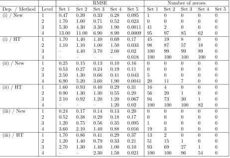
Table 1 displays the root mean squared errors (RMSEs) of the log of all non-zero estimated probabilities. For our model, we define a probability to be zero if its estimate is less than twice machine epsilon in R, since numerical procedures are involved in the calculations; this can occasionally produce negative numbers, which we also set to zero. The number of probabilities estimated as zero is also provided in the table. Overall the new model produces estimates with lower RMSEs than the Heffernan–Tawn model. Any exceptions arise when the Heffernan–Tawn model estimates only a very few non-zero probabilities. In general, estimation for sets closer to one of the axes is better when the dependence is lower. This seems natural as when dependence is high, few if any points in a dataset will be observed near the axes. Both models perform poorly under strong dependence for sets near the axes. Future work could explore whether a more sophisticated implementation of our approach, such as allowing differentfV, k · km, or changing the censoring scheme, improves this.
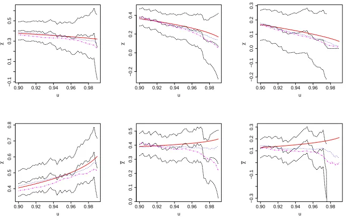
As a diagnostic for the model fit, we also consider the extremal dependence functions χ(u), defined in Section 4.3, and ¯χ(u) := 2 log(1−u)/log{P(F1(Z1)> u, F2(Z2)> u)} −1 foru∈(0.9,0.999) (Coles et al.,
1999). As u →1, χ(u)→ χ, as in (1.1), whilst ¯χ(u) → χ¯ = 2η−1 ∈ [−1,1]. The value ofχ thus gives some discrimination between different asymptotically dependent copulas, whilst ¯χcan discriminate between different asymptotically independent copulas. As functions ofu,χ(u) and ¯χ(u) are useful for checking model fits under either dependence scenario. In the Supplementary Material, Figure 1 displays pointwise medians and 90% confidence intervals ofχ(u),χ¯(u) for each dependence structure and for both methods of inference. Small biases of the new model are typically offset by lower variability and better performance away from the diagonal, i.e., away from the region on whichχ(u) and ¯χ(u) focus.
6
Environmental application
We consider an oceanographic dataset comprising measurements of wave height, surge and wave period recorded at Newlyn, U.K., filtered to correspond to a 15-hour time window for approximate temporal in-dependence, and previously analyzed by Coles and Tawn (1994), Bortot et al. (2000) and Coles and Pauli (2002). Coles and Tawn (1994) noted the presence of seasonality, which was not taken into account in their, or subsequent, analyses; for ease of comparison we also ignore it. Coles and Tawn (1994) used an asymp-totically dependent model for these data, whilst Bortot et al. (2000) used an asympasymp-totically independent Gaussian tail model. Coles and Pauli (2002) employed a mixture-type model, able to encompass both de-pendence types, with asymptotic dede-pendence arising at a boundary point. The literature appears to have reached a consensus that there is strong, but not overwhelming, evidence for asymptotic dependence between wave height and surge, and fairly strong evidence for asymptotic independence between the other two pairs. Here we fit the simple symmetric model (5.2), with dependence threshold u= 0.95 in likelihood (5.1). Marginal transformations to uniformity were carried out using the semiparametric procedure of Coles and Tawn (1991) described in Section 5.1, but the dependence parameter estimates were almost the same using the fully empirical marginal transformation.
Table 2 gives maximum likelihood estimates and confidence intervals for the dependence parameters. The estimate ˆλ = 0.54 suggests asymptotic dependence between wave height and surge, whilst the values ˆ
Table 1: RMSEs of non-zero log-probabilities and number of zero estimated probabilities for the new model (New) and Heffernan and Tawn model (HT) for dependence structures (i)–(iii).
RMSE Number of zeroes
Dep. / Method Level Set 1 Set 2 Set 3 Set 4 Set 5 Set 1 Set 2 Set 3 Set 4 Set 5
(i) / New 1 0.47 0.39 0.33 0.28 0.095 1 0 0 0 0
2 1.70 1.00 0.71 0.52 0.023 0 0 0 0 0
3 5.30 4.30 3.30 1.90 0.0011 41 2 0 0 0
4 13.00 11.00 6.90 8.90 0.0009 95 97 85 62 0
(i) / HT 1 1.70 1.40 1.40 0.69 0.17 45 19 8 0 0
2 1.10 1.10 1.00 1.50 0.033 98 87 57 18 0
3 – 4.40 3.70 2.00 0.02 100 99 99 89 0
4 – – – – 0.018 100 100 100 100 0
(ii) / New 1 0.25 0.15 0.13 0.10 0.16 0 0 0 0 0
2 0.53 0.27 0.24 0.19 0.11 0 0 0 0 0
3 2.50 1.30 0.66 0.41 0.043 5 0 0 0 0
4 6.90 5.20 3.60 1.90 0.0041 20 11 7 0 0
(ii) / HT 1 1.60 0.93 0.40 0.29 0.31 16 4 0 0 0
2 0.90 1.30 1.30 0.55 0.20 56 20 1 0 0
3 2.10 0.92 1.20 1.20 0.067 94 73 30 1 0
4 – – – 1.20 0.02 100 100 100 82 0
(iii) / New 1 0.24 0.17 0.14 0.13 0.20 0 0 0 0 0
2 0.52 0.38 0.29 0.18 0.17 0 0 0 0 0
3 1.20 0.75 0.56 0.35 0.095 1 0 0 0 0
4 3.60 2.10 1.40 0.88 0.016 19 3 0 0 0
(iii) / HT 1 1.70 0.86 0.41 0.29 0.37 13 2 0 0 0
2 1.20 1.40 0.79 0.33 0.21 51 15 1 0 0
3 2.70 1.30 1.40 1.00 0.10 93 69 27 1 0
4 – – 2.30 1.50 0.021 100 100 96 54 0
Table 2: Maximum likelihood estimates and 95% profile likelihood confidence intervals for (λ, α), for the pairs of oceanographic variables.
Height–Surge Height–Period Surge–Period
ˆ
λ 0.54 (0.26,0.90) −0.21 (−0.40,−0.03) −0.43 (−0.66,−0.16) ˆ
α 0.58 (0.40,0.81) 2.21 (1.58,3.06) 0.68 (0.50,0.90)
by the confidence intervals. The likelihood surfaces plotted in Figure 1 show that the parameters are identifiable and give an appreciation of the joint asymptotic confidence regions. Figure 2 shows the empirical and fitted functions χ(u) and ¯χ(u), which suggest a reasonable fit to the data. Fits from the Heffernan– Tawn model are also displayed, conditioned on each variable in turn, and show potential discrepancies in the inferred strength of the dependence; by having only a single model, we can avoid such discrepancies and the need to decide which variable should be chosen for conditioning upon.
A further diagnostic is presented in Figures 3 (a) and (b), where “fitted” values of ˆS= max( ˆA,Bˆ), and ˆ
V = ˆA/( ˆA+ ˆB) are plotted for the pairs height–surge and period–surge, on a uniform scale. Plots for height– period are similar to those for period–surge, and hence are omitted. Here ( ˆA,Bˆ) = [ ˆFA−1{F˜1(Z1)},FˆB−1{F˜2(Z2)}],
where ˆFA = ˆFB is the fitted common pseudo-marginal distribution, and ˜F1,F˜2 are the estimated true
marginals. Points are plotted corresponding to ( ˆS,Vˆ) where ˆSexceeds its 90% quantile. A lack of discernible patterns in Figures 3 (a) and (b) suggests that independence ofSandV is a reasonable approximation. For comparison, Figures 3 (c) and (d) show equivalent plots with max(XP, YP) andXP/(XP+YP) on a uniform
scale, (XP, YP) = [{1−F˜1(Z1)}−1,{1−F˜2(Z2)}−1]; this would be the approach to modelling under
[image:13.612.137.461.464.502.2]is plausible, but that a higher threshold is required for independence of max(XP, YP) and XP/(XP+YP).
Figure 3 (d) shows that these variables would be dependent at any finite threshold.
7
Extensions and discussion
We have provided an alternative limit representation for bivariate extremes, which motivates a statistical model that can capture a wide spectrum of asymptotically dependent and asymptotically independent be-haviour. An obvious question concerns extensions to higher dimensions. Assumption (1.4) is indeed simple to extend to the multivariate case: in some common margins, F, the vector of positive random variables
X= (X1, . . . , Xk) = [F−1{F1(Z1)}, . . . , F−1{Fk(Zk)}] satisfies
lim
t→∞P
X
Pk
i=1Xi
≤w,kXk∗> a(t)r+b(t)
kXk∗> b(t) !
=J(w) ¯K(r), r≥0, (7.1)
at continuity points of J, withJ placing mass on the interior of S1
k−1 ={w ∈Rk+ :kwk1= 1}, and ¯K as
in (1.5). This is a more general assumption than multivariate regular variation, thek-dimensional extension of (1.3), that underpins much of classical multivariate extreme value theory (de Haan and de Ronde, 1998). However, the practical applicability of assumption (7.1) in higher dimensions is more limited than in the bivariate case. The assumption that the distribution of W := X/Pk
i=1Xi has mass on the interior
of S1
k−1 requires a certain regularity in the multivariate dependence structure, which is present in many
theoretical examples, such as in the multivariate extensions of Examples 1–3, but often absent in datasets. For example, the data analyzed in Section 6 exhibited asymptotic dependence between one pair of variables, but asymptotic independence between the other two pairs. The only existing model which can handle this is that of Heffernan and Tawn (2004). However there are obvious issues with the curse of dimensionality when using a semiparametric model for higher dimensions. The simulation study in Section 5 demonstrated a tendency for the semiparametric distribution estimator not to cover all parts of the plane, and this drawback would be exacerbated in higher dimensions.
We have assumed throughout that the radial variable R = k(X, Y)k∗ is defined by a norm, following
the development of much of classical multivariate extreme value theory. In fact the convexity property does not appear necessary, and some recent articles on multivariate extremes have shifted focus on to positive homogeneous functions rather than norms (e.g. Dombry and Ribatet, 2015; Scheffler and Stoev, 2015). For our model the convexity property of k · kmwas used in some of the derivations; further work could explore
more deeply the consequences of relaxing this assumption.
A simple extension to the practical modelling introduced in Sections 5 and 6 is to allow an asymmetric dependence structure. Our theoretical results in Section 4 already cover this scenario, but for simplicity of implementation we assumed the distribution of V to be symmetric, so that the pseudo-marginals of A, B
were equal. As noted in Remark 1, the impliedH incorporates the necessary moment constraint for anyFV.
In essence our approach is intermediate between assuming multivariate regular variation and the ap-proach of Heffernan and Tawn (2004). With the former, both the marginal distribution and the form of the normalization of each marginal variable, i.e.,XP/kXPk, are fixed. This is restrictive, but allows for simpler
characterization of the consequences of the assumption. With the latter, the margins are fixed to be of exponential type, but the form of the normalization of each marginal variable,{XE−b(YE)}/a(YE), is not
fixed. This permits great flexibility in the variety of distributions that satisfy the assumption, but leavesk
possible limits, each with 2(k−1) parameters to estimate, and a (k−1)-dimensional empirical distribution. Our main assumption does not fix the form of the margins, but does fix the form of the normalization of the variablesX/kXk∗. This offers greater flexibility than multivariate regular variation, and although less
flexible than the model of Heffernan and Tawn (2004) has the benefit of giving only a single limit. In the bivariate case, model (4.1), inspired by (1.4), permits inference across both extremal dependence classes, with a smooth transition between them.
Acknowledgements
λ
α
0.2 0.4 0.6 0.8 1.0
0.3 0.4 0.5 0.6 0.7 0.8 0.9 1.0 X λ α
−0.5 −0.4 −0.3 −0.2 −0.1 0.0 0.1
1.5 2.0 2.5 3.0 X λ α
−0.7 −0.6 −0.5 −0.4 −0.3 −0.2 −0.1
[image:15.612.94.514.86.212.2]0.4 0.5 0.6 0.7 0.8 0.9 1.0 X
Figure 1: Negative log-likelihood surfaces for height–surge, height–period and surge–period, respectively. Contours are in steps of 0.5. Crosses show maximum likelihood estimates.
0.90 0.92 0.94 0.96 0.98
−0.1 0.1 0.3 0.5 u χ
0.90 0.92 0.94 0.96 0.98
−0.2 0.0 0.2 0.4 u χ
0.90 0.92 0.94 0.96 0.98
−0.2 −0.1 0.0 0.1 0.2 0.3 u χ
0.90 0.92 0.94 0.96 0.98
0.4 0.5 0.6 0.7 0.8 u χ
0.90 0.92 0.94 0.96 0.98
0.0 0.1 0.2 0.3 0.4 0.5 u χ
0.90 0.92 0.94 0.96 0.98
[image:15.612.130.475.273.490.2]−0.3 −0.1 0.1 0.2 0.3 u χ
Figure 2: Empirical (dashed lines, with approximate 95% pointwise confidence intervals) and fitted (solid line) estimates ofχ(u) (top row) and ¯χ(u) (bottom row), foru∈(0.9,0.99). From left to right the pairs are height–surge, height–period and period–surge. Dot-dash lines: Heffernan–Tawn fit conditioning on the first variable of the pair. Dotted lines: Heffernan–Tawn fit conditioning on the second variable of the pair.
0.0 0.2 0.4 0.6 0.8 1.0
0.0 0.2 0.4 0.6 0.8 1.0 Uniform V Unif or m S (a)
0.0 0.2 0.4 0.6 0.8 1.0
0.0 0.2 0.4 0.6 0.8 1.0 Uniform V Unif or m S (b)
0.0 0.2 0.4 0.6 0.8 1.0
0.0 0.2 0.4 0.6 0.8 1.0
Uniform XP+YPXP
Unif
or
m max(
XP YP
)
(c)
0.0 0.2 0.4 0.6 0.8 1.0
0.0 0.2 0.4 0.6 0.8 1.0
Uniform XP+YPXP
Unif
or
m max(
XP YP
)
(d)
Figure 3: Fitted ˆS and ˆV, on a uniform scale, for (a) height–surge, and (b) period–surge. For comparison, max(XP, YP) and XP/(XP +YP) defined from the variables transformed to a standard Pareto scale are
given for the same pairs in (c) and (d), respectively. Points which are aligned on the ˆS / max(XP, YP) axis
[image:15.612.116.492.570.658.2]greatly improved the work.
A
Auxiliary results and proofs
A.1
Link between
(1.4)
and
(3.2)
Proposition 5. Let W = X/(X+Y), R = k(X, Y)k∗, and assume thatW and R have a joint density.
Further assumeR to be in the domain of attraction of a generalized Pareto distribution, with normalization functionsa(t)>0,b(t). Then, provided that the limit on the right exists,
lim
t→∞P{W ≤w, R > a(t)r+b(t)|R > b(t)}=J(w) ¯K(r) ⇔ tlim→∞P{W ≤w|R=b(t)}=J(w).
Proof. Right to left: The statement on the right is equivalent to
lim
t→∞
∂
∂b(t)P{W ≤w, R > b(t)}
∂
∂b(t)P{R > b(t)}
=J(w).
Since both limt→∞P{W ≤w, R > b(t)}and limt→∞P{R > b(t)}equal zero, but the ratio of the derivatives
has limitJ(w), the general form of l’Hˆopital’s rule states that
lim
t→∞
P{W ≤w, R > b(t)}
P{R > b(t)} =J(w).
Consequently, ast→ ∞,
P{W ≤w, R > a(t)r+b(t)| R > b(t)}= P{W ≤w, R > a(t)r+b(t)}
P{R > a(t)r+b(t)}
P{R > a(t)r+b(t)}
P{R > b(t)} →J(w) ¯K(r).
Left to right: Setr= 0 in the left-hand statement, yielding
lim
t→∞
P{W ≤w, R > b(t)}
P{R > b(t)} =J(w) ¯K(0),
and note that ¯K(0) = 1. Then applying l’Hˆopital’s rule again provides
lim
t→∞
∂
∂b(t)P{W ≤w, R > b(t)}
∂
∂b(t)P{R > b(t)}
=J(w).
A.2
Proofs of Propositions 1–4
We prove Propositions 1–4, giving the values of χ, η and κ claimed in Section 4.2. Omitted proofs of Lemmas 1 and 2, and Propositions 6, 7, 8 and 9 are provided in the Supplementary Material. The following lemma on inversion of regularly varying functions will be useful throughout.
Lemma 1. Suppose β >0 and φis a slowly varying function such that s7→s−βφ(s) defines a continuous
strictly decreasing function from[s0,∞)onto(0,1]for somes0. Then we can find a slowly varying function
u defined on [1,∞) such that s−βφ(s) =t−β whenever s =tu1/β(t). Furthermore u(t)→ c as t → ∞iff φ(s)→c ass→ ∞(here ccan be any value in the extended range [0,+∞]).
The slowly varying functionsφ−1/β andu1/β are de Bruijn conjugates.
Define τ : [0,1] → [1,∞] as the reciprocal of T : [0,1] → [0,1] defined in Section 4.2, i.e., τ(v) =
k(v,1−v)km/v, so thatτ(V) = 1/V1 andτ(1−V) = 1/V2. Using this notation equation (4.3) becomes
P(A > x) =
Z 1
0
{1 +λxτ(v)}−+1/λdFV(v), P(B > y) =
Z 1
0
where the upper endpoint of the support is Λ = +∞ifλ≥0 and Λ =−1/λifλ <0; and (4.4) becomes
P(A > x, B > y) =
Z 1
0
1 +λmax{xτ(v), yτ(1−v)}−1/λ
+ dFV(v) (A.2a)
=
Z x/(x+y)
0
{1 +λxτ(v)}+−1/λdFV(v) +
Z 1
x/(x+y)
{1 +λyτ(1−v)}+−1/λdFV(v). (A.2b)
The expressionsx7→P(A > x) andy7→P(B > y) define continuous strictly decreasing functions from [0,Λ) onto (0,1]; this observation can be used to help justify the conditions for Lemma 1 when it is used below.
From Condition 2, τ(v)≥(1−v)/v >1 forv <1/2, while Conditions 1 and 3 imply τ(v) = 1 for some
v∈[1/2,1]. Set Ω0={v∈[0,1] :τ(v) = 1}. Nowτ(v) = ˜τ(1/v) where ˜τ : [1,∞]→[1,∞] is the continuous
convex function defined by ˜τ(u) = k(1, u−1)km. It follows that Ω0 is a closed subinterval of [1/2,1], so
Ω0= [v0, v00] withv0,v00as defined in Section 4.2. Also note that 1/2≤v0≤v00≤1,
τ is strictly decreasing on [0, v0] and strictly increasing on [v00,1], (A.3) and
v≶ x
x+y ⇐⇒ yv≶x(1−v) ⇐⇒ yτ(1−v)≶xτ(v). (A.4)
The quantitiesm+ andm− as given in Proposition 4 can be expressed
m+=
Z
Ω0
dFV(v) =FV(v00)−FV(v0) and m−= Z
1−Ω0
dFV(v) =FV(1−v0)−FV(1−v00);
by Assumption 1, m+, m− >0 iff v0 6=v00. We proceed with Cases 1–3 in turn, firstly by establishing the
form of the quantile functionsqA(tβ) andqB(tγ), followed by proofs of the main Propositions concerning the
behaviour of the joint survivor functions.
A.2.1 Case 1: λ >0
Recall the positive quantitiesµ1, µ2defined in Remark 1; these can be expressedµ1=λ−1/λR 1 0 τ
−1/λ(v) dF V(v),
andµ2=λ−1/λR 1 0 τ
−1/λ(1−v) dF V(v).
Proposition 6. Let β, γ >0. Then there exist slowly varying functions lA,lB such that qA(tβ) =tλβlA(t)
andqB(tγ) =tλγlB(t)for allt≥1. Furthermore lA(t)→µλ1 andlB(t)→µλ2 ast→ ∞.
Proof of Proposition 1. Firstly supposeβ=γ. From (A.2a),θβ,γ as defined in Proposition 1, is
θβ,γ(t) =
Z 1
0
t−λβ+λmax{lA(t)τ(v), lB(t)τ(1−v)}
−1/λ
+ dFV(v).
Sinceτ ≥1, andlA(t) (orlB(t)) has a non-zero limit ast→ ∞, we can bound max{lA(t)τ(v), lB(t)τ(1−v)}
uniformly away from 0 for all sufficiently larget. Furthermore Proposition 6 implies max{lA(t)τ(v), lB(t)τ(1−
v)} →max{µλ
1τ(v), µλ2τ(1−v)}ast→ ∞. Applying dominated convergence and using the definitions ofµ1
andµ2 then gives
lim
t→∞θβ,γ(t) =
Z 1
0
λmax{µλ1τ(v), µ
λ
2τ(1−v)}
−1/λ
dFV(v) =χλ.
The fact that this limit is non-zero impliesθβ,γ is slowly varying. Now assume β < γ (the caseβ > γ can
be handled similarly). Then
r(t) := qA(t
β)
qA(tβ) +qB(tγ)
=n1 +tλ(γ−β)lB(t) lA(t)
o−1
→0, t→ ∞.
Ifv≤r(t) then (A.4) gives
qA(tβ)τ(v)≥qB(tγ)τ(1−v) =⇒ 1 +λqA(tβ)τ(v)≥1 +λqB(tγ)τ(1−v)> λqB(tγ)>0
=⇒ 0<
1 +λqB(tγ)τ(1−v)
−1/λ
+ −
1 +λqA(tβ)τ(v)
−1/λ
+ ≤
λqB(tγ)
−1/λ
Combined with (A.1) and (A.2b) we thus have
0≤P{B > qB(tγ)} −P
A > qA(tβ), B > qB(tγ)
=
Z r(t)
0
1 +λqB(tγ)τ(1−v)
−1/λ
+ −
1 +λqA(tβ)τ(v)
−1/λ
+
dFV(v)
≤
Z r(t)
0
{λqB(tγ)}−1/λdFV(v) =t−γ{λlB(t)}−1/λFV{r(t)}.
The continuity ofFV at 0 givesFV{r(t)} →FV(0) = 0 as t→ ∞. SinceP{B > qB(tγ)}=t−γ we then get
P{A > qA(tβ), B > qB(tγ)}=t−γ{1 +o(1)} ast→ ∞. The result follows.
Proof of Proposition 2. Note that by Condition 3,v00>1/2. From (4.5) we getχλ≤ R−+R+ where
R−=
R1/2
0 τ
−1/λ(v) dF V(v)
R1
0 τ−
1/λ(v) dF V(v)
and R+=
R1
1/2τ
−1/λ(1−v) dF V(v)
R1
0 τ−
1/λ(1−v) dF V(v)
.
Nowτ(v)≥1 with equality iffv∈Ω0. Since Ω0⊆[1/2,1] dominated convergence then gives
lim
λ→0+
Z 1/2
0
τ−1/λ(v) dFV(v) = 0 and lim λ→0+
Z 1
0
τ−1/λ(v) dFV(v) =
Z
Ω0
dFV(v) =m+.
Ifv0 = 1/2< v00 thenm+>0 soR−→0 asλ→0+. Otherwisev0 >1/2, in which case we can findδ >0
so thatτ(v)≥1 +δwhenv∈[0,1/2]. SettingIδ ={v∈[0,1] :τ(v)≤1 +δ/2}we then get
R−≤
R1/2
0 (1 +δ)
−1/λdF V(v)
R
Iδ(1 +δ/2)
−1/λdF V(v)
≤ (1 +δ)
−1/λ
(1 +δ/2)−1/λC δ
=Cδ−1ρ1/λ
whereρ= 1−δ/(2 + 2δ)∈(0,1) andCδ :=RI
δ dFV(v)>0 (positivity follows from Assumption 1 and the
fact that the interval length|Iδ|>0). Asλ→0+,ρ1/λ→0 and henceR−→0. A similar argument shows
R+→0.
A.2.2 Case 2: λ= 0
Letβ, γ >0 and setω=β/(β+γ)∈(0,1). Thenβτ(ω) =k(β, γ)km=γτ(1−ω) while (A.4) gives
ν(v) := max{βτ(v), γτ(1−v)}=
(
βτ(v) if 0≤v≤ω,
γτ(1−v) ifω≤v≤1. (A.5)
The function ν is a positive, continuous and convex function on [0,1], with ν(0) = +∞ = ν(1). Set
b
ν := min{ν(v) : v ∈ [0,1]} and Ω := {v ∈ [0,1] : ν(v) = νb}; in particular, Ω is a non-empty closed subinterval of [0,1]. The general shape ofν and key properties ofνband Ω can be deduced from (A.3):
C1: ω∈[1−v0, v0]. Thenβτ(v) is strictly decreasing on [0, ω],γτ(1−v) is strictly increasing on [ω,1] and
these quantities are equal whenv=ω. It follows that Ω ={ω}andbν=βτ(ω) =γτ(1−ω) =k(β, γ)km.
C2: ω ∈(v0,1). Thenν(v) =βτ(v) is strictly decreasing on [0, v0] andν(v) =βτ(v) =β (a constant) on [v0,min{ω, v00}]. Alsoβτ(v) is strictly increasing on [v00,1] andω > v0≥1−v0 so γτ(1−v) is strictly increasing and not less thanβτ(v) on [ω,1]; henceν(v) = max{βτ(v), γτ(1−v)}is strictly increasing on [min{ω, v00},1]. It follows that Ω = [v0,min{ω, v00}] andνb=β=k(β, γ)k∞(note that,ω > v0 ≥1/2
which impliesβ > γ).
C3: ω∈(0,1−v0). By a similar argument toC2, Ω = [max{ω,1−v00},1−v0] andνb=γ=k(β, γ)k∞.
Lemma 2. Suppose a : [0,1] → [0,∞] is continuous, u is regularly varying at infinity with index ρ > 0, andI, Is⊆[0,1] fors≥0 is a collection of closed intervals with the interval length|I|>0 andIs→I as
s→ ∞. Define φ by
φ(s) =
Z
Is
u−a(v)(s)dFV(v)
for eachs≥0, and setα= min{a(v) :v∈I}. Thenφ is regularly varying with index−αρ.
Note that byIs→Iwe mean that the Hausdorff distance betweenIsandItends to 0; equivalently, the
end points ofIsconverge to the end points ofI.
Proposition 7. Let β, γ > 0. Then there exist slowly varying functions lA, lB such that qA(tβ) =
log{tβlA(t)} and qB(tγ) = log{tγlB(t)} for all t ≥ 1. Furthermore lA, lB are continuous, take values in
[m+,1]and[m−,1]respectively, and satisfylA(t)→m+ andlB(t)→m− ast→ ∞.
Proof of Proposition 3. Setting
r(t) = qA(t
β)
qA(tβ) +qB(tγ)
= βlogt+ loglA(t) (β+γ) logt+ loglA(t)lB(t)
(A.6)
we haver(t)→ω ast→ ∞(note thatlA andlB are slowly varying). Furthermore (A.2b) gives
P
A > qA(tβ), B > qB(tγ) =
Z r(t)
0
e−τ(v) log{tβlA(t)}dF
V(v) +
Z 1
r(t)
e−τ(1−v) log{tγlB(t)}dF
V(v)
=
Z r(t)
0
tβlA(t)
−τ(v)
dFV(v) +
Z 1
r(t)
tγlB(t)
−τ(1−v)
dFV(v). (A.7)
Now assume β ≤ γ (the case β ≥ γ can be handled similarly). Then ω ≤ 1/2 ≤ v0 so (A.3) gives min{τ(v) : v ∈ [0, ω]} = τ(ω) = k(β, γ)km/β. Furthermore, Ω ⊆ [ω,1] (recall the description of ν at
the beginning of this section) so min{τ(1−v) :v∈[ω,1]}=γ−1min{ν(v) :v∈[ω,1]}=bν/γ. Lemma 2 can now be applied to show that the integrals on the right hand side of (A.7) are regularly varying functions, the first with index−k(β, γ)km≤ −νband the second with index −νb. By the forms of bν described inC1–C3
immediately preceding Lemma 2, the result follows.
The fact thatχ= 0 when η= 1 in this case is given by the following.
Proposition 8. Ifv0 6=v00 (equivalently m+, m−>0) and 1−v0≤ω≤v0 then limt→∞θβ,γ(t) = 0.
A.2.3 Case 3: λ <0, k(1,1)km=k(1,1)k∞, with Assumption 2
Proposition 9. Letβ, γ >0. Then there exist slowly varying functionslA,lBsuch thatqA(tβ) = Λ−tλβlA(t)
andqB(tγ) = Λ−tλγlB(t) for allt≥1. FurthermorelA(t)→Λmλ+ andlB(t)→Λmλ− ast→ ∞.
Let ∆ be a neighbourhood of 1/2 on whichFV0 is continuous; in particular, dFV(v) =FV0 (v) dvforv∈∆.
Proof of Proposition 4. Setr(t) =qA(tβ)/{qA(tβ) +qB(tγ)}so (A.2b) gives P
A > qA(tβ), B > qB(tγ) =
I−+I+ where
I−=
Z r(t)
0
{1 +λqA(tβ)τ(v)}−
1/λ
+ dFV(v) and I+=
Z 1
r(t)
{1 +λqB(tγ)τ(1−v)}−
1/λ
+ dFV(v).
To consider I− firstly set v−(t) = qA(tβ)/{qA(tβ) + Λ}. Since qB(tγ) < Λ and qA(tβ), qB(tγ) → Λ as
t→ ∞we get v−(t)< r(t) while v−(t), r(t)→1/2 as t→ ∞. Asv00>1/2 we can then chooseT0 so that
[v−(t), r(t)]⊆[1−v00, v00]∩∆ whenevert ≥T0. Fort≥T0 it follows that τ(v) = max{(1−v)/v,1} when
v∈[v−(t), r(t)]; in particularτ{v−(t)}= Λ/qA(tβ). Furthermore (A.3) impliesτ(v) is decreasing on [0, r(t)].
Forv∈[v−(t), r(t)] we thus have
1 +λqA(tβ)τ(v)>0 =⇒ τ(v)<
1
−λqA(tβ)