An asynchronous method for cloud based rendering

warwick.ac.uk/lib-publications

Manuscript version: Author’s Accepted Manuscript

The version presented in WRAP is the author’s accepted manuscript and may differ from the

published version or Version of Record.

Persistent WRAP URL:

http://wrap.warwick.ac.uk/108585

How to cite:

Please refer to published version for the most recent bibliographic citation information.

If a published version is known of, the repository item page linked to above, will contain

details on accessing it.

Copyright and reuse:

The Warwick Research Archive Portal (WRAP) makes this work by researchers of the

University of Warwick available open access under the following conditions.

Copyright © and all moral rights to the version of the paper presented here belong to the

individual author(s) and/or other copyright owners. To the extent reasonable and

practicable the material made available in WRAP has been checked for eligibility before

being made available.

Copies of full items can be used for personal research or study, educational, or not-for-profit

purposes without prior permission or charge. Provided that the authors, title and full

bibliographic details are credited, a hyperlink and/or URL is given for the original metadata

page and the content is not changed in any way.

Publisher’s statement:

Please refer to the repository item page, publisher’s statement section, for further

information.

(will be inserted by the editor)

An asynchronous method for cloud-based rendering

Keith Bugeja · Kurt Debattista · Sandro Spina

Received: date / Accepted: date

Abstract Interactive high-fidelity rendering is still un-achievable on many consumer devices. Cloud gaming services have shown promise in delivering interactive graphics beyond the individual capabilities of user de-vices. However, a number of shortcomings are mani-fest in these systems: high network bandwidths are re-quired for higher resolutions and input lag due to net-work fluctuations heavily disrupts user experience. In this paper we present a scalable solution for interactive high-fidelity graphics based on a distributed rendering pipeline where direct lighting is computed on the client device and indirect lighting in the cloud. The client device keeps a local cache for indirect lighting which is asynchronously updated using an object space rep-resentation; this allows us to achieve interactive rates that are unconstrained by network performance for a wide range of display resolutions that are also robust to input lag. Furthermore, in multi-user environments, the computation of indirect lighting is amortised over participating clients.

Keywords Rendering·Rasterization·Global Illumi-nation_·Distributed Algorithms_·Cloud Computing

1 Introduction

An accurate lighting model and rapid visual feedback are two important factors in conveying realistic graph-ics at interactive rates [33][41]. While a large number of methods for computing realtime dynamic global illumi-nation have been proposed, increasing the level of im-mersion in virtual environments, these typically trade

K. Bugeja

Department of Computer Science, University of Malta

E-mail: [email protected]

off quality and accuracy for performance, and are inca-pable of running on all but the most powerful machines.

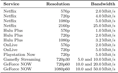
Table 1: Bandwidth requirements/recommendations for various video-on-demand and cloud gaming services.

Service Resolution Bandwidth

Netflix 576p 2.0 Mbit/s

Netflix 720p 4.0 Mbit/s

Netflix 1080p 5.0 Mbit/s

Netflix 2160p 25.0 Mbit/s

Hulu Plus 576p 1.0 Mbit/s

Hulu Plus 720p 2.0 Mbit/s

Hulu Plus 1080p 3.2 Mbit/s

OnLive 576p 2.0 Mbit/s

OnLive 720p 5.0 Mbit/s

Playstation Now 720p 5.0 Mbit/s

Gamefly Streaming 720p30 5.0 and 10.0 Mbit/s

GeForce NOW 720p60 10.0 and 20.0 Mbit/s

GeForce NOW 1080p60 10.0 and 50.0 Mbit/s

Typical cloud gaming systems, commercial ones also, employ a straightforward offloading strategy where each connecting client is synchronously mapped to a single cloud server running the desired application. Virtualised environments are oftentimes employed for less computationally-demanding applications such as legacy titles. Application output is then streamed back to the client as video [10]. Besides lacking the scalability required of economic cloud deployments, this approach does not take advantage of amortisation of computation since each server works in isolation.

This paper proposes Remote Asynchronous Indi-rect Lighting (RAIL), a distributed rendering technique that decouples inexpensive computations from the rest of the rendering pipeline and moves their execution to the client device. Through asynchronous computation, the system provides highly responsive high-fidelity ren-dering at HD resolutions and higher, and makes use of amortisation of computation to deliver improved scala-bility for multiple users sharing the same virtual envi-ronments [8]. The contributions of this work are:

– a scalable asynchronous distributed rendering method with low bandwidth requirements that is resolution-independent and robust to network ser-vice fluctuations, expected of typical connectivity over the Internet;

– the application of the method to the software-as-a-service (SaaS) paradigm for highly interactive ren-dering in HD (and higher) over a wide spectrum of devices.

2 Related Work

Dachsbacher et al. [12] present a survey of many-lights algorithms, a class of global illumination methods inspired by Instant Radiosity [22], a bidirectional

rendering technique that emits rays from light sources and follows them as they interact with surfaces across the scene. At every ray-surface interaction, a virtual point light (VPL) is created, to approximate the indirect lighting contribution of the surface region centred at the point of intersection. Both direct and indirect lighting computation are reduced to a single operation, the summation of contributions from point light sources dotted across the scene. Debattista et al. [15] introduced a hybrid of Instant Radiosity [22] and the Irradiance Cache [42], which is conceptually similar to the shading method proposed in this work, albeit the former is view-dependent. Bikker et al. [6] present a method to generate a view-independent point cloud for storing shading information; we use a similar method to generate a representation for static scene geometry, which is adequate to demonstrate the con-cept of remote asynchronous rendering. Nevertheless, RAIL is not tied to a specific generation algorithm and more efficient ones may be used if so desired.

them a viable option due to the laborious nature of the parameterisation [10]. Photon tracing doesn’t require any parameterisations but has substantially larger bandwidth requirements, close to an order of magnitude more than the requirements of streaming cloud gaming platforms. Moreover, the indirect lighting reconstruction at the client poses prohibitive compu-tational costs for some low to mid-range devices. The third algorithm, which adopts a synchronous approach, uses cone-traced sparse voxel global illumination, and although updates at 30 Hz can be sustained for 5 clients, this soon drops to 12 Hz as soon as the number of clients is increased to 24. Liu et al. [27] propose a distributed rendering pipeline which, similarly to Cloudlight [10], streams GI information to the client us-ing H.264 encoded video. Indirect lightus-ing is computed using view-dependent techniques, such as reflective shadow maps [13], light propagation volumes [21] and voxel cone tracing [11]; thus, computation cannot be amortised across multiple clients and camera changes require GI to be recomputed.

3 Method

The goal of RAIL is to provide high-fidelity graphics that go beyond the capabilities of individual client de-vices, and to do so at highly interactive rates with min-imal bandwidth requirements and input lag, which has been shown to be detrimental to user experience.

In high-fidelity rendering, dynamic indirect lighting comprises a substantial part of the computational cost of frame synthesis, beyond the means of most consumer devices. Conversely, direct lighting, can be adequately computed by most consumer devices furnished with ba-sic hardware graphics capabilities, from smartphones to tablets, to laptops to desktop machines. These sys-tems are equally capable of visualising precomputed indirect illumination, typically reconstructing it from view-independent data structures.

RAIL decouples direct and indirect lighting, computing the latter in the cloud. Indirect lighting is stored in a view-independent data structure, a snapshot of which is also kept by the client and asynchronously updated. This snapshot is used to reconstruct indirect lighting at every frame, whenever direct lighting is computed by the client. This method has a number of advantages: (i) visual fidelity may go beyond the computational possibilities of a client device in isolation;(ii) frame updates are not bound to network performance, eliminating any input lag; and (iii) a server-based view-independent indirect lighting representation can be shared among multiple clients

collaborating within a virtual environment, possibly amortising computation costs.

Algorithm 1Synchronous version of the proposed ren-dering algorithm.

1: Q←GeneratePointSet(scene) .(§3.1)

2: whiletruedo

3: V ←TraceVPLs(scene) .(§3.2)

4: ShadePointSet(Q, V) .(§3.2)

5: I←ReconstructIndirect(scene, Q) .(§3.2)

6: D←ComputeDirect(scene)

7: MergeAndPresent(I, D) .(§3.3)

8: end while

Although RAIL is designed as an asynchronous dis-tributed rendering algorithm (see Figure 1), for clarity we initially present a synchronous centralised formula-tion of the algorithm, elaborating on how a point de-scription of the scene is generated and used to com-pute indirect lighting for object surfaces and recon-struct the full global illumination solution in realtime (see Algorithm 1). Briefly, a point cloud representation of the scene is generated offline for sampling diffuse in-direct lighting (line 1). Light tracing is used to gener-ate VPLs (line 3), which are used to shade the gen-erated point cloud (line 4). Indirect lighting is recon-structed from the sparse samples in the point cloud (line 5) and merged with the direct lighting component (lines 6-7). In the reconstruction of indirect lighting, static geometry (non-movable, non-deformable geome-try) is shaded using interpolated irradiance from the point cloud (§3.3), while dynamic geometry is shaded using a higher-order ambient function, a coarse approx-imation of indirect lighting (§3.4). The asynchronous distributed formulation of the algorithm is introduced subsequently, in Section 4.

3.1 Generation of Diffuse Indirect Sample Point Set

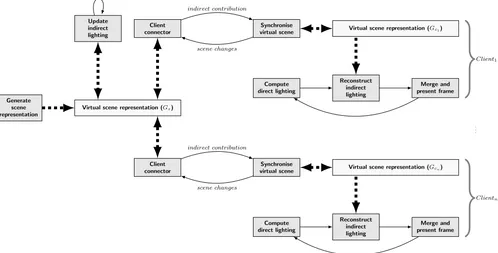
Virtual scene representation (Gs)

Virtual scene representation (Gc1)

Virtual scene representation (Gcn)

Generate scene representation

Update indirect lighting

Client connector

Synchronise virtual scene

scene changes indirect contribution

Compute direct lighting

Reconstruct indirect lighting

Merge and present frame

Client1

Client connector

Synchronise virtual scene

scene changes indirect contribution

Compute direct lighting

Reconstruct indirect lighting

Merge and present frame

Clientn

. . .

Fig. 1: Rendering using remote asynchronous computation, high-level architecture

The area of effect of a dart, or record, is determined by evaluating the ambient occlusion function at the respective point in the scene [24].

3.2 Estimation and Reconstruction of Indirect Lighting

The estimation of indirect lighting is a dynamic process that is affected by scene changes in illumination sources or objects. This entails evaluating the rendering equa-tion [20] over the hemisphere centred at each sample point. To accomplish this, we use a many-lights algo-rithm [12]; specifically, we compute the indirect lighting contribution in two phases, first by tracing a number of light paths and creating VPLs for each path vertex, and secondly by iterating over the VPLs and computing the respective contribution for each unoccluded sample point. The indirect lighting contribution at a point is progressively accumulated when no changes in the scene state are recorded. Specifically, fornprogressive contri-butions, the indirect lighting at the sample point is the mean of these contributionsE = (Pn

i=1Ei)/ n, where Ei is the ith contribution and E the current indirect lighting at an arbitrary sample point. When a change in scene state is effected, a new sequence of contributions is started, to match changes in state. However, to avoid abrupt changes in the lighting, the first term of the new sequence is carried over from the previous sequence

(E0=E). Although this introduces additional bias, it

also favours temporal coherence and shows less discon-tinuity. The estimation step updates a point cloud Q

such that each sample point q_∈Q represents a point on a surface at which diffuse indirect lighting has been evaluated. To reconstruct the indirect lighting function for a pointpon any surface in the scene, an inverse dis-tance weighting is used to interpolate the irregularly-spaced data in Q [39]. The weight of the contribution of each sampleqin the extrapolation of pis given by:

W(p,q) = (max(0, r_{− |}pp−qp|) max(0,pn·qn))µ, (1)

whereris the range determiningq’s area of effect and, pp,qpandpn,qnare the positions and surface normals at p and q respectively. The exponent µ determines whether the reconstruction functionΦpeaks (0< µ≤

1) or is level (µ >1) at the nodes [35]:

Φ(p) =

P

q∈QW(p,q)qe

P

q∈QW(p, q)

. (2)

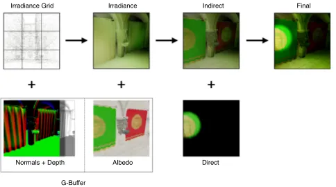
Fig. 2: Parallel view of geometry (left) and generated point sets (right) for the scenes used in this work.

Irradiance Grid Irradiance Indirect Final

Direct Albedo

Normals + Depth

G-Buffer

Fig. 3: The client rendering pipeline reconstructs indi-rect lighting from the shading point cloud and G-buffer, merging the result with direct lighting to obtain a GI solution.

3.3 Integrating Direct and Indirect Lighting

Reconstructing the indirect lighting contribution requires knowledge of point cloud Q and geometric details about the points for which the function is being reconstructed, such as surface positions, normals and albedos. In deferred shading pipelines, which perform screen-space shading, this information is readily available as a geometry-buffer (G-buffer) [16][38]. This makes reconstruction using Equation 2 straightfor-ward but inefficient, since all points in Q have to be considered, even though they might not contribute anything to the final value. Thus, a multiple-reference regular grid G is introduced as an overlay on Q to accelerate nearest neighbour queries using spatial hashing. Records are referenced from each cell that overlaps their sphere of validity, simplifying the lookup to the examination of a single cell and the records contained within.

From equations 1 and 2, it follows that in order to calculate the contribution of each sampleq, properties

like position, surface normal, irradiance and range are required and thus, have to be accounted for in the space complexity of the regular grid. Specifically, letcbe the number of cells along an edge of the grid and c3 _the

total number of cells in the grid. The edge of each cell is cl units long. The sample range of effect r in the weighting function (Equation 1) determines the spatial extent of a search operation and can be used to estimate the maximum number of references for a sample to (2r/ cl)3_{, with the total being}

|Q_{| ·}(2r / cl)3_{. Each cell holds}

an index to a record reference, which points to the first record in a bin that holds references to records affecting the given cell. A further indirection exists, that maps each reference to the actual record index, and finally the records themselves are stored. The index held in each cell of the grid is 4 bytes long, while each entry in the reference map is 8 bytes long. A single record is 23 bytes long, 12 bytes for position, 8 for surface normals and 3 for irradiance. The upper bound on the space requirements of the regular grid is thus |Q| ·(8(2r / cl)3_{+ 23) + 4c}3_{. A typical grid (c = 64, c}

l = 4, r = 6 and_|Q_|= 40000) requires 10 MB of GPU memory.

these cases, prior to the final composition, geometry-aware upscaling using joint bilateral upsampling [23] is applied to the channel. Similarly to McGuire et al. [30], the weights used are based on 2D bilinear interpolation, normals and depth differences between the low and high resolution G-buffers. The upscaled irradiance is combined with the albedo channel and then with the direct contribution, to derive the final image (Figure 3).

Algorithm 2Propagation of ambient contribution val-ues to empty cells.

1: procedurePropagate(grid,iterations) 2: Ac[· · ·]←1

3: for1≤n≤iterationsdo

4: for each p∈grid∧ ¬isEmpty(p)do

5: cells←FilterNeighbours(p) 6: for each c∈cells∧isEmpty(c)do

7: Ae[c]←Ae[c] +Ae[p]

8: inc Ac[c]

9: end for

10: end for

11: for each p∈griddo

12: Ae[p]←Ae[p]/Ac[p]

13: end for

14: end for

15: end procedure

16: procedureFilterNeighbours(p)

17: n←An[p]

18: cells← ∅

19: for eachaxis∈ {x, y, z}do

20: if |naxis|>= √1

3 then

21: nsgn=sgn(naxis)

22: cells←cells∪neighbour(p, axis, nsgn)

23: end if

24: end for

25: returncells

26: end procedure

3.4 Dynamic Scenes

The system currently supports dynamic objects, de-formable ones also. These objects are factored in the VPL tracing and point cloud shading steps (§3.2), and thus, can occlude and reflect light. To avoid chang-ing the structure of the grid G (see §3.3) whenever an object moves, a coarser approximation of indirect lighting is used, inspired by ambient occlusion, and is computed in two steps. The constant ambient term, traditionally used to approximate indirect reflections in the scene, is turned into a higher-order function of space; this is then evaluated by partitioning the scene into a coarse regular grid, with each cell containing an ambient term approximation for the region, and tri-linearly interpolating these values across adjacent cells

(see§3.5). The ambient term for each cell is computed from the weighted mean of all irradiance points in Q

affecting the cell. This coarse grid is referred to as the

ambient grid A, and is distinct from the grid G dis-cussed in Section 3.3; the latter is used to accelerate nearest neighbour searches of Q. Spatially, A is fitted over scene geometry such that the longest edge of the bounding volume of the scene corresponds to an edge of the bounding volume of A. The edges of the ambi-ent grid are equal, which means that, geometrically, it is a cube, subdivided equally along all edges. The con-stituting cells contain three important values, a single quantityAerepresenting the weighted mean irradiance (ambient contribution) of the sample points inQwhich are also contained with the volume of the cell itself, a normalised vectorAn representing the principal direc-tion of the sample normals contained within the cell, and a scalar contribution countAc that keeps track of the number of ambient contributions a given cell has received from neighbouring cells. Cells are indexed via a triplep= (x, y, z), where 0≤x, y, z < subdivisions. The ambient contribution for a cell is computed as fol-lows:

Ae[x, y, z] =

P

q∈Qxyzqoqe P

q∈Qxyzqo

, (3)

whereQxyzis the subset of points inQthat is contained in the grid cell with index (x, y, z), and qe and qo are the irradiance and ambient occlusion values for sample qrespectively. Note thatqois computed offline, during the generation ofQ, and stored (see§3.1). The layout of scene geometry, and consequently the distribution ofQ, may be such that some cells in the grid are empty (i.e.,

Qxyz=∅). A straightforward iterative approach is used to propagate the ambient contribution from neighbour-ing cells and fill empty ones. When the ambient grid is first created, principal component analysis is performed on the normal vectors of the samples contained in each cell. A principal component is determined and used as the aggregated surface normal An for that cell. Prop-agation is a runtime process which uses the ambient contribution values of neighbouring cells to populate the empty ones; the process is described in Algorithm 2. For each cell in the grid that has a valid ambient contribution (source cell), the direction of propagation is determined from the principal normalAn. The nor-mal is used to determine which neighbouring cells to consider. The principal normaln=Ap[px, py, pz] is de-composed into its axial componentsnx, ny and nz. If the length of each component exceeds a given threshold (_±√1

3), then the cells adjacent to the face with the

Consequently, the ambient contribution of the source cell is combined with that at each of the selected neigh-bours; Ac keeps track of the number of contributions a cell has received during one iteration of propagation. An iteration completes once all the source cells have been considered, after which the propagated contribu-tions are averaged. Figure 4 gives an example of propa-gation, for two iterations. The threshold value _√1

3 is the

length of each component of a unit vector which makes an angle ofπ/4 to each principal axis.

3.5 Using the Ambient Grid

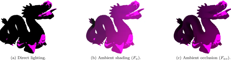
During rendering, the ambient grid A is used to con-tribute indirect lighting to regions that are not covered by the samples in Q, such as dynamic geometry. Ir-radiance at p is coarsely estimated from the ambient contributions by performing trilinear interpolation be-tween adjacent cells of the grid, denoted by Fa(A,p). The application of Fa to geometry subject only to di-rect lighting can be seen in figures 5a and 5b. In the first figure, the object is illuminated only by means of direct light; since the light is partially occluded, a great part of the object is depicted in black. In the second fig-ure the black patches on the object are now lit via the ambient function, albeit the latter does not take into ac-count surface occlusion. Thus, a heavily occluded point receives the same contribution as one that is less oc-cluded, leading to a loss of perception of the shape of the object, as can be observed in Figure 5b. In order to curtail a point’s exposure to ambient lighting and pro-vide a better perception of the shape of geometry [24], ambient occlusion (AO) is applied toFa. The extension to the ambient function is thus:

Fao(A,p) = Fa(A,p)

π Z

Ω

V(p, ω)ω_·Np dω. (4)

AO being a global method, it requires access to scene geometry in order to compute point visibility, which makes it less suitable for use in rasterisation. Instead of traditional AO, screen space ambient occlusion (SSAO) is used, which is a faster approximation that computes occlusion from neighbouring pixel depths rather than scene geometry [32]. The application of the new ambi-ent function Fao can be seen in Figure 5c, where the AO term is evaluated using SSAO.

4 Distributing the Rendering Pipeline

In this section, the synchronous rendering method described thus far is transformed into an asynchronous distributed rendering pipeline (see Algorithm 1).

The first three steps (lines 1-4) are computationally expensive, beyond the reach of low-end hardware such as smartphones and tablet devices, making them good candidates for offloading to a powerful server backend. Particularly, the first step (line 1), which generates the point set, is a one-time precomputation step that can be carried out offline. The last two steps (lines 5-7) may be easily run on a low-end device, provided

Q is available, in the form of the regular grid G

(see §3.3). Distributing the rendering pipeline, thus, becomes a problem of synchronisation, whereby the regular grids at client ends are made consistent with that at the server, and the server’s representation of dynamic objects in the scene, such as light sources, is made consistent with that of its clients. The highly interactive nature of client applications precludes the use of a blocking synchronisation mechanism that depends on network performance. Thus, a particular gridGc at a client device is treated as a local cache of the server version Gs, and is updated asynchronously, without affecting the local rendering steps (lines 5-7), which are allowed to run unconstrained. Server-side,

Gs is updated to reflect indirect diffuse lighting in the scene (3-4) and executes independently of client communication. Any scene changes received from clients are queued and applied to scene state on the server, invalidating indirect lighting computed thus far (see Figure 1).

4.1 Synchronisation of Indirect Lighting

(a) No ambient value.

Ae[i−1, j+ 1] Ae[i, j+ 1]

(b) 1st_iteration.

Ae[i−1, j+ 1] Ae[i, j+ 1]

(c) 2nd _iteration.

Fig. 4: Iterative propagation process for ambient lighting. In 4a, cells that contain no samples (and hence no ambient value) are marked in white. Ae[i, j] marks the weighted mean of irradiance values, which is used to propagate indirect lighting to adjacent cells. In 4b, one iteration of propagation has been performed, and the empty cells adjacent to (i, j) which face the hemisphere of directions aroundAn[i, j] have received indirect lighting. Particularly, An[i, j] acts as an occluder of sorts, to stop propagating values in its opposite direction. Cells that do not have a normal vector defined due to being empty of irradiance samples propagate values in all directions, that is, to all empty adjacent cells. 4c shows the ambient grid after two iterations of propagation, where all the empty cells are now populated with an ambient value.

(a) Direct lighting. (b) Ambient shading (Fa). (c) Ambient occlusion (Fao).

Fig. 5: Indirect lighting function for dynamic objects, where 5a is the base direct lighting, 5b shows the object shaded with the spatially-varying ambient term, and 5c augments 5b with screen space ambient occlusion.

transfers between the server and a client. Messages are packed using an LZF compressor [25], for a reduction in size of up to 40%.

4.2 Two-stage smoothing

The indirect lighting synchronisation process is asyn-chronous and can run at a lower frequency than the client rendering. In some scenes it can be very difficult to generate paths between light sources and the cam-era [4], requiring a larger number of VPLs to be traced for a more accurate estimation of indirect lighting [14]. This situation is exacerbated when the light sources are moving and any accumulated contribution has to

be constantly reset, leading to artefacts and flickering. To reduce flickering and the disparity between direct and indirect lighting update rates, a simple two-stage smoothing mechanism is used. The first stage uses ex-ponential averaging to combine the current irradiance values in Gc with the newly received values from Gs such that for every sample, E0

c = wcEc+ (1−wc)Es, whereE0

illumination may be perceived to be lagging behind the direct illumination. The weightwc can be adjusted at runtime and is typically initialised to 0.5. An attempt has been made to basewc on the change in orientation of the observer, with large changes resulting in a smaller weight and vice versa, and although preliminary results look promising this has not been formally evaluated. The second smoothing stage is used to compensate for the difference in update frequencies between direct and indirect lighting. For an arbitrary sample, the irradi-ance value used in the previous frame to reconstruct indirect lighting (Ed) and the most recent update for that same sample (Ec) are linearly interpolated to give the impression that irradiance is updating at the same rate as direct lighting. Let Er(t) be an interpolation function:

Er(t) =



  

  

Ed t≤0

Er(0) + t

∆T(Er(∆T)−Er(0)) 0< t < ∆T

Ec t≥∆T

(5)

where t ∈ [0, ∆T) is the time elapsed since the last cache update (Gc = Gs), ∆T is the interval to the next cache update; the frequency of cache updates de-termine how quickly Ed approaches Ec. The interval length to the next cache update, ∆T, is not known a priori, therefore it is estimated using an exponential average function:

∆Tn+1=wd ∆Tn+ (1−wd)τn, (6)

where τ n is the recorded interval for the nth _update,

∆Tn is the estimated interval for the nth update, and

wd∈[0,1] determines whether more weight is given to the previous estimate or the actual reading when com-puting the next estimate. Forwc = 1, the next estimate is based entirely on previous estimates,∆Tn+1=∆Tn;

for wd = 0, the next estimate becomes the length of the last recorded interval, ∆Tn+1 = τn. ∆T0 is set to

100 ms. In an ideal scenario where no network and com-munication fluctuations are present, a small value of

wd will quickly converge to a constant update interval. Nevertheless, even on an ideal network, the messages exchanged by client and server are still expected to vary in size since the amount of data transferred is propor-tional to the number of irradiance samples contained in the view frustum of the observer (see§4.1). Empiri-cally, values ofwd in the interval [0.55,0.8] were found to give the best results and produce less variance in the estimations, in the general case (see §5.1).

4.3 Amortisation of Computation

The virtual scene representation used for rendering is available on both the server and the connected clients. The server needs this information to be able to compute indirect lighting, while the clients require the scene for local rendering, including the reconstruction of indirect lighting and possibly any additional application logic that manipulates the objects within. A client that changes the scene representation by moving objects or lights, for instance, is responsible for informing the server (see Figure 1) and initiating the synchronisation process to ensure the scene is consistent at both ends. The point setQ, which is the representation of diffuse indirect lighting in the virtual scene, is updated once for all connected clients that share the same multi-user environment. Notwithstanding any possible work repli-cation due to scene synchronisation mentioned above, the centralised indirect lighting computation outweighs the penalties thereof; not only are these costs quickly amortised, but the more clients participating in the same virtual environment, the greater the benefits in terms of computation sharing, which result in a form of speed-up.

5 Results

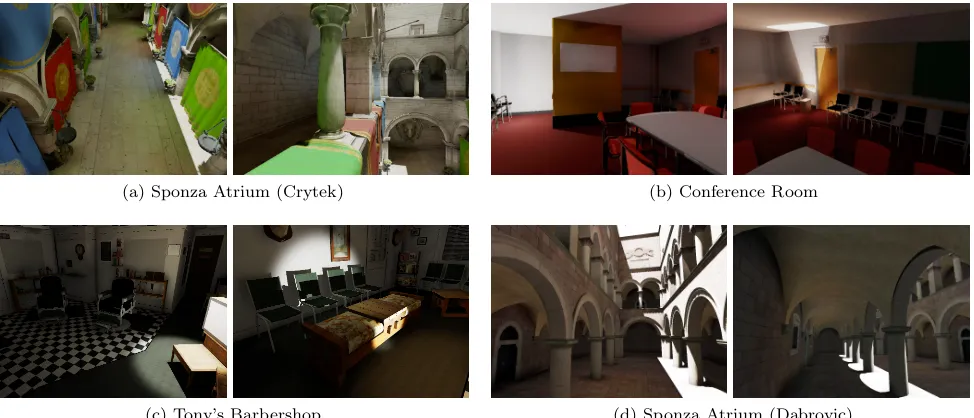
The following results address the scalability of the sys-tem, both at client and server-side, bandwidth require-ments, latency, and the respective error incurred due to these networking constraints. The system has been tested on four scenes, Sponza Atrium (both the original version and Crytek’s), Tony’s Barbershop (a Half-Life 2 death match community map), and Conference Room. The Barbershop data set was introduced because be-sides being a traditional interactive raster scene, it is densely populated with geometric detail from small ob-jects. The generated point cloud representation sizes for the maps were 14.5 k, 21.5 k, 32 k and 38.6 k points re-spectively. The parameters for the production of these point sets were empirically determined to strike a bal-ance between quality and performbal-ance, in terms of both computation and communication. In Figure 7, the cell distribution per sample point in a 323 _{grid is shown; it}

(a) Sponza Atrium (Crytek) (b) Conference Room

(c) Tony’s Barbershop (d) Sponza Atrium (Dabrovic)

Fig. 6: The scenes used for remote rendering using asynchronous computation.

1 3 10 30

0 2,000 4,000 6,000

Cells

Barber Conf.

Crytek Dabr.

(a) Unique samples.

1 3 10 30

0 2,000 4,000 6,000

Sample Count

Cells

Barber Conf.

Crytek Dabr.

(b) Samples with radius overlapping multiple cells.

Fig. 7: Plot of cell frequency counts against the number of contained samples in a grid with 323 _{cells. In 7(a),}

no duplicate (multiple-referenced) samples are shown; in 7(b), samples that overlap multiple cells are included in each of the cells.

of RAM and an NVIDIA GeForce GTX 680 display adapter. The server-side implementation uses NVIDIA OptiX to accelerate VPL shooting and occlusion test-ing. The client-side implementation has been carried out in Unity3D; reconstruction shaders were written in Direct Compute and thus require Direct3D11-capable hardware.

0 0.2 0.4 0.6 0.8 1

20 40 60

Interpolation Weight (wd)

Error

(

σ

)

Unmod. s= 16

s= 32 s= 64

Fig. 8: Standard deviation for prediction error.

5.1 Preliminaries

The values for two-stage smoothing (see§4.2) were set to wc = 0.5 for the first and wd = 0.65 for the sec-ond stage respectively. The value for the secsec-ond stage was determined experimentally; a sequence of one hun-dred cache update intervalsτi. . . τi+99was sampled and

the estimation error (∆Tn−τn) was recorded forwd∈

{0,0.05,0.1, . . . ,0.95,1_}. To simulate fluctuations both

in the network and communication, the recorded inter-vals were modulated by a sinusoidal function:

τn0 =τn

sin2nπ

s Xn+ 1

, (7)

error for the interval sequences. From the graph, it can be seen that the interpolation weights yielding less variance on average lie in the range [0.55,0.8]. Taking the mean of the error values for each individual weight in the range returns the lowest value at wd = 0.65; this value is used in the following results. The band-width (§5.2) and image-fidelity (§5.4) results have been recorded over a scripted set of paths, one for each of the four scenes, since it was necessary to replicate the camera movement over multiple runs of the experiment.

5.2 Bandwidth

The bandwidth requirements of the system have been recorded for all scenes: 2.826 Mbit/s for Bar-bershop; 1.712 Mbit/s for Conference; 1.54 Mbit/s and 1.159 Mbit/s for Sponza Crytek and Dabrovic respectively. In this test, both the camera view and the light sources followed a scripted path wherein they were constantly changing, precluding any quiescence that could have been achieved by scenes that change very infrequently or in bursts. The client and server complete a roundtrip exchange of indirect lighting at an average frequency of 6 Hz. The total bandwidth requirements do not exceed 3 Mbit/s, which is on the same level as the minimum recommendations for game streaming services (see Table 1), but for the fact that our system is resolution invariant, and reconstructing UHD quality images requires no additional bandwidth. High-dynamic-range (HDR) streaming requires higher bandwidth allocations, depending on the numerical precision allotted to each colour channel; bandwidth requirements double and quadruple for 16-bit (half-float) and 32-bit (single precision) colour ranges respectively. Comparatively, Netflix for in-stance, requires 25 Mbit/s to stream in HDR, which is twice the estimated bandwidth required by RAIL. It is worth pointing out that although the Barbershop scene has a smaller point cloud than the Conference scene, it is nonetheless more densely populated. This results in a larger number of points captured by frustum culling when compared to the other scenes, which also reflects in the higher bandwidth requirements. Notwithstand-ing, these requirements are lower than most game streaming requirements for even 720p resolutions. The results highlight the potential of achieving high-fidelity graphics on resources of varying computational power without compromising interactivity response times due to network fluctuations and bandwidth constraints. The method scales adequately at both ends of the hardware spectrum, on average achieving frame rates of approximately 25 Hz at a resolution of 1024_×768 on the Intel Atom tablet, and over 60 Hz at UHD

1 2 4 8 16 24

100 200 300

Resp

onse

time

(ms)

Barber Conf. Crytek Dabr.

(a) Changes in response times for tested scenes as the number of clients increases - a measure of scalability.

1 2 4 8 16 24

102 103

Indirect

(ms)

Ideal Seq. Par.

(b) Mean indirect lighting computation scalability for ideal parallel, sequential and actual parallel runs.

1 2 4 8 16 24

0 10 20

Clients

Sp

eed-up

Ideal Barber Conf. Crytek Dabr.

(c) Speed-up in the computation of indirect lighting due to amor-tisation.

Fig. 9: Scalability and performance evaluation results showing system behaviour in terms of response times and indirect lighting computational overhead as the number of connected clients increases.

resolutions on a desktop PC equipped with a GeForce GTX680. The obvious bottleneck during rendering is the reconstruction of indirect lighting, where for each pixel shaded, a nearest neighbour search has to be carried out. Since the system employs a multi-reference grid, the entire set of samples contributing to indirect lighting are contained within a single cell; from Figure 7(b) it becomes evident that the majority of cells contain at most 10 samples.

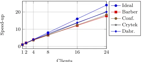
5.3 Client Scalability (Remote System Overhead)

in an increased communication latency between clients and the server-end, when streaming indirect lighting. Updates follow a request-response model, where the client initiates each update itself; this request-response cycle has been measured for all test scenes with a vary-ing number of clients and it was found that the in-crease in latency for up to 24 clients is almost negligi-ble, suggesting that the system is capable of scaling well beyond this number (see Figure 9a). Figure 9b shows the amortisation of computation for the indirect diffuse component, in each of the four scenes. If the computa-tion were to be decentralised and moved back to each individual client, for a homogeneous group of clients c

where each member is working individually, the amount of work done would increase by a factor ofc₋1. Fort

ms of original computation time on the server, the to-tal work for c independent clients would increase toct

ms. In RAIL, indirect lighting computation is valid for all connected clients, and thus, the ideal computation time would be t as opposed to ct. However, Figure 9a highlights the fact that realisation penalties exist that are introduced due to communication and synchronisa-tion, and increase as more clients are added. To account for them, the actual computation time forc clients be-comes rp(c) +t, where rp(c) is the realisation penalty forc clients. Figure 9b shows mean plots for t (Ideal),

rp(c) +t (Par.) andct(Seq.) for all four scenes. Figure 9c expresses this gain in terms of computation speed-up; it must be stressed that the gain comes at no cost since the clients would otherwise still have to perform the computation of indirect lighting themselves.

5.4 Image fidelity

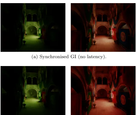
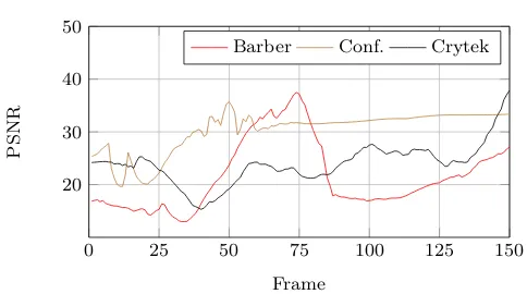
The remote asynchronous nature of RAIL introduces temporal discrepancies between the direct and indirect lighting components. In this test we measure image fidelity as a function of these discrepancies; particu-larly, we measure the difference between a typical and a zero-latency execution of the system, the latter gen-erated entirely and synchronously on the server using the rendering method described in Section 3, without any time constraints. For both methods, scripted walk-throughs over three of the test scenes were rendered and compared. The light sources and camera view change throughout all but the end of the animation, where the image was allowed to converge over a number of frames. Figure 10 shows two selected image pairs from the gen-erated walkthroughs; their structured similarity (SSIM) index is 0.9429 and 0.8165 for the left and right pair re-spectively. The peak signal-to-noise ratio (PSNR) was computed for each pair of frames in the resulting ani-mations; this is shown in Figure 11.

(a) Synchronised GI (no latency).

(b) Asynchronous indirect lighting.

(c) Difference images.

Fig. 10: A comparison between zero-latency (10a) and asynchronous indirect lighting (10b). The latter con-tributes to output lag, where the indirect lighting ap-pears to trail behind the direct lighting. The differences between the two pair of images are shown in Figure 10c. The structural similarity (SSIM) index is 0.9429 for the left image pair and 0.8165 for the right.

5.5 Limitiations and future directions

0 25 50 75 100 125 150 20

30 40 50

Frame

PSNR

Barber Conf. Crytek

Fig. 11: PSNR values characterising latency of indirect lighting over animation sequences for tested scenes.

the generated sizes of point sets, an overly dense data set may result in higher bandwidth usage as well as longer computation times at the server-end, for the estimation of indirect lighting. This is suggested by the bandwidth usage and the request-response cycle times of Figure 9a. The grid implementation itself is straightforward; the memory arrangement avoids interleaving of data to speed up copies during updates. However, during the reconstruction phase, when cells are constantly being queried, memory access patterns have not been profiled to detect any sub-optimal behaviour. The process could be further studied to see if there is still potential for optimisation. Since scene point-cloud generation is a one-time precom-putation step, dart throwing and na¨ıve Poisson disk sampling were employed [6]; however, other more efficient strategies and approaches could be used, with desirable properties such as the generation of maximal distributions [18]. Blue noise sampling strategies [40], [3], [37] may also be investigated due to their improved convergence rate over other samplers, including Poisson disk sampling, during Monte Carlo integration [36]; the application of these strategies to the domains of geometry representation and reconstruction may lead towards improved solutions that yield better coverage or faster convergence.

6 Conclusion

The results highlight the potential of achieving high-fidelity graphics on resources of varying computational power without compromising interactivity response times due to network fluctuations and bandwidth constraints. Server-side scalability is very promising, with minimal overhead incurred when increasing the number of clients. The scalability results in Figure 9b show that additional clients in multi-user environments can be added at very little cost, since indirect lighting

is amortised over them. This carries a significant advantage over streaming solutions which provide each of the clients with rendering sandboxes that do not interact and thus, share no computation load. While other cloud methods have been presented, both as fully streaming solutions and as distributed rendering pipelines, our solution requires lower bandwidth and is robust to latency. Furthermore, with respect to purely streaming solutions, our method can amortise the computation of indirect lighting in multi-user environments with minimal costs for each additional client.

References

1. Autodesk 360 (2014). URL

http://www.autodesk.com/products/rendering/overview

2. renderrocket (2014). URL

http://www.renderrocket.com/features/

3. Ahmed, A.G., Niese, T., Huang, H., Deussen, O.: An adaptive point sampler on a regular lattice. ACM

Trans-actions on Graphics (TOG)36(4), 138 (2017)

4. Bashford-Rogers, T., Debattista, K., Chalmers, A.: Im-portance driven environment map sampling (2013)

5. Bierton, D.: Face-off: Gaikai vs. onlive (2012). URL

http://www.eurogamer.net/articles/digitalfoundry-face-off-gaikai-vs-onlive

6. Bikker, J., Reijerse, R.: A precalculated point set for

caching shading information. In: Eurographics

2009-Short Papers, pp. 65–68. The Eurographics Association (2009)

7. Brouillat, J., Gautron, P., Bouatouch, K.: Photon-driven irradiance cache. In: Computer Graphics Forum, vol. 27, pp. 1971–1978. Wiley Online Library (2008)

8. Bugeja, K., Debattista, K., Spina, S., Chalmers, A.: Col-laborative high-fidelity rendering over peer-to-peer net-works. In: Eurographics Symposium on Parallel Graphics and Visualization, pp. 9–16. The Eurographics Associa-tion (2014)

9. Chalmers, A., Reinhard, E., Davis, T.: Practical parallel rendering. CRC Press (2002)

10. Crassin, C., Luebke, D., Mara, M., McGuire, M., Os-ter, B., Shirley, P., Sloan, P.P., Wyman, C.: Cloud-Light: A system for amortizing indirect lighting in

real-time rendering. Journal of Computer

Graph-ics Techniques (JCGT) 4(4), 1–27 (2015). URL

http://jcgt.org/published/0004/04/01/

11. Crassin, C., Neyret, F., Sainz, M., Green, S., Eisemann, E.: Interactive indirect illumination using voxel cone trac-ing. In: Computer Graphics Forum, vol. 30, pp. 1921– 1930. Wiley Online Library (2011)

12. Dachsbacher, C., Kˇriv´anek, J., Haˇsan, M., Arbree, A.,

Walter, B., Nov´ak, J.: Scalable realistic rendering with

many-light methods. In: Computer Graphics Forum,

vol. 33, pp. 88–104. Wiley Online Library (2014) 13. Dachsbacher, C., Stamminger, M.: Reflective shadow

maps. In: Proceedings of the 2005 symposium on Inter-active 3D graphics and games, pp. 203–231. ACM (2005) 14. Dammertz, H., Keller, A., Lensch, H.P.: Progressive

point-light-based global illumination. In: Computer

15. Debattista, K., Dubla, P., Banterle, F., Santos, L.P., Chalmers, A.: Instant caching for interactive global il-lumination. In: Computer Graphics Forum, vol. 28, pp. 2216–2228. Wiley Online Library (2009)

16. Deering, M., Winner, S., Schediwy, B., Duffy, C., Hunt, N.: The triangle processor and normal vector shader: a vlsi system for high performance graphics. In: ACM SIG-GRAPH Computer Graphics, vol. 22, pp. 21–30. ACM (1988)

17. Dipp´e, M.A., Wold, E.H.: Antialiasing through stochastic

sampling. ACM Siggraph Computer Graphics19(3), 69–

78 (1985)

18. Gamito, M.N., Maddock, S.C.: Accurate

multidimen-sional poisson-disk sampling. ACM Transactions on

Graphics (TOG)29(1), 8 (2009)

19. Jensen, H.W.: Realistic image synthesis using photon mapping. AK Peters, Ltd. (2001)

20. Kajiya, J.T.: The rendering equation. In: ACM Siggraph Computer Graphics, vol. 20, pp. 143–150. ACM (1986) 21. Kaplanyan, A., Dachsbacher, C.: Cascaded light

propaga-tion volumes for real-time indirect illuminapropaga-tion. In: Pro-ceedings of the 2010 ACM SIGGRAPH symposium on Interactive 3D Graphics and Games, pp. 99–107. ACM (2010)

22. Keller, A.: Instant radiosity. In: Proceedings of the 24th annual conference on Computer graphics and interactive techniques, pp. 49–56. ACM Press/Addison-Wesley Pub-lishing Co. (1997)

23. Kopf, J., Cohen, M.F., Lischinski, D., Uyttendaele, M.:

Joint bilateral upsampling. In: ACM Transactions on

Graphics (TOG), vol. 26, p. 96. ACM (2007)

24. Langer, M.S., B¨ulthoff, H.H.: Depth discrimination from

shading under diffuse lighting. Perception29(6), 649–660

(1999)

25. Lehmann, M.A.: Lzf compression library (liblzf) (2014). URL http://www.goof.com/pcg/marc/liblzf.html 26. Lewis, M.: The new cards. Communications of the ACM

45(1), 30–31 (2002)

27. Liu, C., Jia, J., Zhang, Q., Zhao, L.: Lightweight web-sim rendering framework based on cloud-baking. In: Pro-ceedings of the 2017 ACM SIGSIM Conference on Princi-ples of Advanced Discrete Simulation, pp. 221–229. ACM (2017)

28. Manzano, M., Hern´andez, J.A., Uruen˜na, M., Calle, E.:

An empirical study of cloud gaming. In: Proceedings

of the 11th Annual Workshop on Network and Systems Support for Games, p. 17. IEEE Press (2012)

29. Mara, M., Luebke, D., McGuire, M.: Toward practical real-time photon mapping: efficient gpu density estima-tion. In: Proceedings of the ACM SIGGRAPH Sympo-sium on Interactive 3D Graphics and Games, pp. 71–78. ACM (2013)

30. McGuire, M., Luebke, D.: Hardware-accelerated

global illumination by image space photon

map-ping. In: Proceedings of the 2009 ACM

SIG-GRAPH/EuroGraphics conference on High Performance

Graphics. ACM, New York, NY, USA (2009). URL

http://graphics.cs.williams.edu/papers/PhotonHPG09/ 31. Mitchell, J., McTaggart, G., Green, C.: Shading in valve’s

source engine. In: ACM SIGGRAPH 2006 Courses, pp. 129–142. ACM (2006)

32. Mittring, M.: Finding next gen: Cryengine 2. In:

ACM SIGGRAPH 2007 Courses, SIGGRAPH

’07, pp. 97–121. ACM, New York, NY, USA

(2007). DOI 10.1145/1281500.1281671. URL

http://doi.acm.org/10.1145/1281500.1281671

33. Myszkowski, K., Tawara, T., Akamine, H., Seidel, H.P.: Perception-guided global illumination solution for anima-tion rendering. In: Proceedings of the 28th annual con-ference on Computer graphics and interactive techniques, pp. 221–230. ACM (2001)

34. Pajak, D., Herzog, R., Eisemann, E., Myszkowski, K., Seidel, H.P.: Scalable remote rendering with depth and motion-flow augmented streaming. In: Computer Graph-ics Forum, vol. 30, pp. 415–424. Wiley Online Library (2011)

35. P´al, L., Ol´ah-G´al, R., Mak´o, Z.: Shepard interpolation

with stationary points. Acta Univ. Sapientiae1(1), 5–13

(2009)

36. Pilleboue, A., Singh, G., Coeurjolly, D., Kazhdan, M., Ostromoukhov, V.: Variance analysis for monte carlo

in-tegration. ACM Transactions on Graphics (TOG)34(4),

124 (2015)

37. Qin, H., Chen, Y., He, J., Chen, B.: Wasserstein blue noise sampling. ACM Transactions on Graphics (TOG)

36(5), 168 (2017)

38. Saito, T., Takahashi, T.: Comprehensible rendering of

3-d shapes. In: ACM SIGGRAPH Computer Graphics,

vol. 24, pp. 197–206. ACM (1990)

39. Shepard, D.: A two-dimensional interpolation function for irregularly-spaced data. In: Proceedings of the 1968 23rd ACM national conference, pp. 517–524. ACM (1968) 40. Wachtel, F., Pilleboue, A., Coeurjolly, D., Breeden, K., Singh, G., Cathelin, G., De Goes, F., Desbrun, M., Os-tromoukhov, V.: Fast tile-based adaptive sampling with

user-specified fourier spectra. ACM Transactions on

Graphics (TOG)33(4), 56 (2014)

41. Walter, B., Drettakis, G., Parker, S.: Interactive render-ing usrender-ing the render cache. In: Renderrender-ing techniques 99, pp. 19–30. Springer (1999)

42. Ward, G.J., Rubinstein, F.M., Clear, R.D.: A ray trac-ing solution for diffuse interreflection. ACM SIGGRAPH