Date of publication xxxx 00, 0000, date of current version xxxx 00, 0000. Digital Object Identifier 10.1109/ACCESS.2017.DOI
Performance Analysis of a Polling Model
with BMAP and Across-Queue
State-Dependent Service Discipline
JIANYU CAO1,2, WEI FENG1,2,3,(Senior Member, IEEE), YUNFEI CHEN4,(Senior Member, IEEE), NING GE1,2,(Member, IEEE), AND SHULAN WANG5
1
Department of Electronic Engineering, Tsinghua University, Beijing 100084, China 2
Beijing National Research Center for Information Science and Technology, Tsinghua University, Beijing 100084, China 3
Peng Cheng Laboratory, Shenzhen 518055, China 4
School of Engineering, University of Warwick, Coventry CV4 7AL, U.K. 5
College of Big Data and Internet, Shenzhen Technology University, Shenzhen 518118, China
Corresponding author: Wei Feng (e-mail: [email protected]).
This work was supported in part by the National Key Research and Development Program of China (Grant No. 2018YFA0701601), in part by the Beijing Natural Science Foundation (Grant No. L172041), in part by the National Natural Science Foundations of China (Grant Nos. 61771286, 61701457, 91638205, 61702341), and in part by the Beijing Innovation Center for Future Chip.
ABSTRACT As various video services become popular, video streaming will dominate the mobile data traffic. The H.264 standard has been widely used for video compression. As the successor to H.264, H.265 can compress video streaming better, hence it is gradually gaining market share. However, in the short term H.264 will not be completely replaced, and will co-exist with H.265. Using H.264 and H.265 standards, three types of frames are generated, and among different types of frames exist dependencies. Since the radio resources are limited, using dependencies and quantities of frames in buffers, an appropriate time division transmission policy can be applied to transmit different types of frames sequentially, in order to avoid the occurrence of video carton or decoding failure. Polling models with batch Markovian arrival process (BMAP) and across-queue state-dependent service discipline are considered to be effective means in the design and optimization of appropriate time division transmission policies. However, the BMAP and across-queue state-dependent service discipline of the polling models lead to the large state space and several coupled state transition processes, which complicate the performance analysis. There have been very few researches in this regard. In this paper, a polling model of this type is analyzed. By constructing a supplementary embedded Markov chain and applying the matrix-analytic method based on the semi-regenerative process, the expressions of important performance measures including the joint queue length distribution, the customer blocking probability and the customer mean waiting time are obtained. The analysis will provide inspiration for analyzing the polling models with BMAP and across-queue state-dependent service discipline, to guide the design and optimization of time division transmission policies for transmitting the video compressed by H.264 and H.265.
INDEX TERMS Across-queue state-dependent, Batch Markovian arrival process, H.264/H.265, polling model, video streaming.
I. INTRODUCTION
W
ITH the fast development in the fields of mobile communications and Internet of Things (IoT) tech-nologies, the number of network access devices is increasing dramatically. Ericsson’s mobility report [1] reveals that, by the end of 2024 there will be 8.9 billion mobile subscriptions, excluding the cellular IoT connections and fixed wireless access subscriptions. Moreover, the video services areI B P B P B I
FIGURE 1. Diagram of the relationship among I-frame, P-frame and B-frame.
radio resources.
The H.264 video compression standard was developed in 2003, and it is suitable for encoding High Definition (HD) video (1920×1080resolution or higher) [2]. Up till now, H.264 has been widely used for video compression. In 2013, the video compression standard H.265 was developed as the successor to H.264. H.265 has better compression for video streaming, and it is suitable for high-resolution compression such as 4K (4096×2160resolution) and 8K (7680×4320 resolution) [3]. Compared with H.264, H.265 can save up to 50% of bandwidth and storage for the same video quality. Nevertheless, the H.265 standard needs more resources to decode or encode. In view of the cost and user’s necessary needs, H.264 will not be completely replaced in the short term, and it will co-exist with H.265. Using H.264 and H.265 standards, three types of frames are generated in video compression, as I-frame (intra frame), P-frame (predictive frame) and B-frame (bi-predictive frame). As shown in Fig. 1, I-frames are complete pictures and don’t require other types of frames to decode; P-frames require I-frames and other frames to decode; B-frames require I-frames and P-frames to decode. If one I-frame is lost, some P-P-frames and B-frames may not be decoded accurately; if one P-frame is lost, some B-frames and other P-frames may not be decoded accurately.
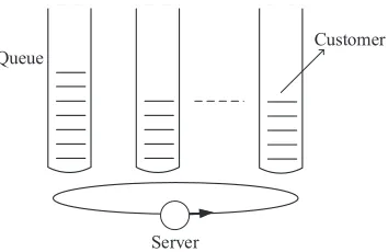
In wireless networks, some devices and data centers are responsible for transmitting the collected or stored video data to the destination. For example, the cameras transmit the collected video data to the processing center through wireless networks, and the cloudlet/fog is deployed on the edge of wireless networks to transmit the stored video to the requesting user. The video data can be compressed by H.264 and H.265 in the upper layer. Due to the dependencies among the generated frames and the limited radio resources, different types of frames can be assigned different transmis-sion priorities, as I-frame >P-frame >B-frame, and they are arranged in different buffers of the data link layer. An appropriate time division transmission policy is implemented in the scheduler to transmit different types of frames orderly. Polling models are considered to be effective means in the design and optimization of time division transmission policies. The classical polling model consists of one serv-er and sevserv-eral queues (see Fig. 2), and the sserv-ervserv-er rendserv-ers services to customers in different queues, according to the
Server
[image:2.576.68.247.66.164.2]Customer Queue
FIGURE 2. Structure of the classical polling model.
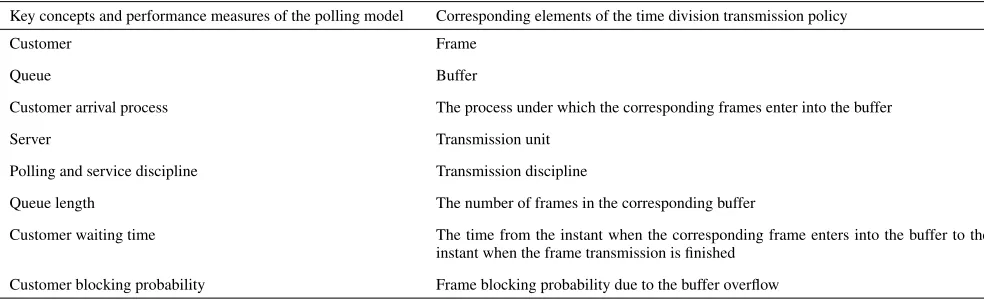
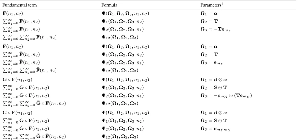
given polling and service discipline. For the key concepts and performance measures, the correspondence between the polling model and the time division transmission policy is shown in Table 1. In this paper, we study the polling model and its performance analysis method which can be used in the design and optimization of time division transmission policies for transmitting the video compressed by H.264 and H.265.
A. RELATED WORKS
Up to now, various polling models have been analyzed. These polling models can be divided into two categories, i.e. ones with intra-queue autonomous service discipline and ones with across-queue state-dependent service discipline, according to whether the service discipline attached to one queue depends on the states of other queues.
1) Polling models with intra-queue autonomous service discipline
In this type of polling models, the service discipline attached to each queue is independent of the states of other queues. For each queue, the common used service disciplines are exhaus-tive, gated, number-limited, time-limited and their variations. Some examples are listed in the following.
TABLE 1. The correspondence between the polling model and the time division transmission policy
Key concepts and performance measures of the polling model Corresponding elements of the time division transmission policy
Customer Frame
Queue Buffer
Customer arrival process The process under which the corresponding frames enter into the buffer
Server Transmission unit
Polling and service discipline Transmission discipline
Queue length The number of frames in the corresponding buffer
Customer waiting time The time from the instant when the corresponding frame enters into the buffer to the instant when the frame transmission is finished
Customer blocking probability Frame blocking probability due to the buffer overflow
In [6], Boxma et al. analyzed the polling model which consists of one server and multiple infinite-buffer queues. The server attends these queues periodically according to a general service order table, and the queues with higher priority are attended frequently. Each queue is attached to one of the three service disciplines, including exhaustive, gated and number-limited (1-limited). For each queue, the numbers of arrivals in every time slots are independent and identically distributed random variables. The pseudoconservation law for this model was derived, and it can be used to obtain approximations for individual mean waiting times. In [7], van Wijk et al. analyzed the polling model which also consists of one server and multiple infinite-buffer queues. The server attends these queues in a cyclic manner, and each queue is served according to the multigated service discipline. The customer arrival processes of the queues are independent Poisson processes. The mean visit time of each queue, the pseudoconservation law, the distribution of waiting times and the mean waiting times were derived.
In [8], Saffer and Telek presented a unified analysis method for the cyclic polling model which consists one server and multiple infinite-buffer queues. The server is entitled to serve the queues in a cyclic manner, and the service disciplines attached to the queues have the following properties: memoryless property, work-conservation proper-ty, non-preemptive service properproper-ty, determination property. The most commonly known disciplines, such as exhaustive, gated, binomial exhaustive, binomial-gated, non-exhaustive, semi-exhaustive, limited-N and non-preemptive limited-T, all satisfy the above properties. The customer arrival process-es of the two queuprocess-es are independent batch Markovian arrival processes (BMAPs) [9].
2) Polling models with across-queue state-dependent service discipline
For this type of polling models, there is at least one queue whose service discipline depends on the states of other queues. Some examples are listed in the following.
In [10], the polling model consists of one server and two infinite-buffer queues. The first queue is served according
to the exhaustive service discipline until it is empty, at this time, if the second queue is not empty, the server switches to the second queue. During the service time of the second queue, (a) if the second queue is not empty while the number of customers in the first queue exceeds a certain threshold, the server switches to the first queue immediately; (b) if the second queue is empty while the number of customers in the first queue does not exceed a certain threshold, the server still switches to the first queue. The customer arrival processes of the queues are independent Poisson processes. The joint queue length distribution was determined.
In [13], Cao and Xie proposed a cyclic polling model with BMAP and across-queue state-dependent service discipline, and analyzed its stability. In this polling model, there are one server and two infinite-buffer queues. The customers arrive at the two queues according to two independent BMAPs; the server is entitled to serve the two queues in a cyclic manner. The customers in the first queue have the higher service priority, and they are served according to the gated service; the customers in the second queue have the lower service priority, and they are served according to the across-queue state-dependent time-limited service discipline. As the length of the first queue increases, the mean predetermined service time of the second queue either decreases or remains the same.
For more polling models, see [14]–[21] and references therein. According to the existing literature, in the current researches on polling models, the customer arrival processes are mostly assumed to be the Poisson processes. For the Poisson arrival process, the customers arrive independently, and the inter arrival times are independent and identically distributed exponential random variables. Hence, the Poisson arrival process can’t effectively describe the arrival charac-teristics of the video streaming that have correlated frames. Fortunately, the BMAP can capture the batch, correlated and bursty nature of the video streaming [22]–[25]. Moreover, it includes the Poisson process, the PH-renewal process, the Markov-modulated Poisson process, the Markovian arrival process as special cases. In addition, the weighted round-robin (WRR) policies are commonly used to transmit data with different priorities [26], [27]. In WRR, the used weights are set statically according to the prior traffic information. In the dynamic weighted round-robin (DWRR), the weights are set dynamically according to the time-varying characteristics of traffic. It was shown in [28], [29] that DWRR can achieve better performance than WRR, without the prior traffic in-formation. Based on this result and the dependencies among the frames generated by H.264 and H.265, it is inferred that the time division transmission policy with across-buffer state-dependent property can effectively improve the transmission quality of the compressed video. The transmission policy attached to one buffer can be dynamically adjusted based on the time-varying characteristics of frames in other buffers with higher priorities. Therefore, the polling models with BMAP and across-queue state-dependent service discipline are worth studying. And they are effective analysis tools to guide the design and optimization of time division transmis-sion policy, for transmitting the video compressed by H.264 and H.265. However, there have been very few researches in this regard. To the best of our knowledge, in 2017, a polling model of this type was proposed firstly [13], and up to now its performance measures have not been analyzed. The method proposed in [8] is not suitable for the model in [13], since the service disciplines need to be independent of the history of the model, whereas in [13], the service time of the second queue depends on the length of the first queue. In [30], Vishnevsky et al. indicated that a polling model can
be analyzed by the decomposition of the polling model into a set of vacation queueing models. But, this method is also not suitable for the model in [13], due to the across-queue state-dependent service discipline attached to the second queue. Indeed, the BMAP and across-queue state-dependent service discipline lead to the large state space and several coupled state transition processes, which complicate the performance analysis.
In this paper, we will analyze the performance of the cyclic polling model, as presented in [13]. The buffer sizes of the two queues are finite in our analysis. The motivation of this paper includes two aspects. First, the performance analysis of the cyclic polling model in this paper can be used as a basis of analyzing the cyclic polling model in [13] with infinite-buffer queues, by increasing the buffer sizes. Second, since the polling models with BMAP and across-queue state-dependent discipline can be used to guide the design and optimization of time division transmission policies for trans-mitting the video compressed by H.264 and H.265, we will explore the method to analyze this type of polling model by concentrating on the two-queue model, whenever possible, suggest extensions to the multi-queue model in the future.
B. OUR MAIN CONTRIBUTIONS
By constructing a supplementary embedded Markov chain and applying the matrix-analytic method based on the semi-regenerative process [31], some important performance mea-sures of the polling model presented are analyzed.
• The expressions of three joint queue length stationary distributions are obtained, including: the joint queue length stationary distribution, at queue 1 polling epochs when the server arrives at the first queue; the joint queue length stationary distribution, at queue 2 polling epochs when the server arrives at the second queue; the joint queue length stationary distribution at arbitrary time. • The expressions of customer blocking probabilities in
different queues are derived.
• The expressions of customer mean waiting times in different queues are obtained.
In addition, the analysis method applied in this paper can provide inspiration for analyzing the polling models with BMAP and across-queue state-dependent service discipline.
C. NOTATIONS
Throughout this paper, unless otherwise stated, notations are used as follows. N = {0,1,2,· · · }; N+ = {1,2,3,· · · };
edenotes a column vector of appropriate size consisting of 1’s; ek (k ∈ N+)denotes a k-dimensional column vector
consisting of 1’s;0denotes a vector or matrix of appropriate size consisting of 0’s;0k (k ∈ N+)denotes ak×kmatrix
consisting of 0’s; 0k1×k2 (k1, k2 ∈ N
+)denotes ak 1×k2
matrix consisting of 0’s; I denotes an identity matrix of appropriate size; Ik (k ∈ N+) denotes a k× k identity
matrix. For anyn1, n2 ∈ N, ifn1 = n2, then δn1,n2 = 1;
{x|x∈Aandx /∈B}. Given a matrix A whose elements (which may be blocks) are indexed by (i, j) ∈ Ω1×Ω2,
where the set Ω1 consists of the row indices which are
all either scalars or row vectors with the same dimension, and the set Ω2 consists of the column indices which are
all either scalars or row vectors with the same dimension,
A can be denoted by A = Ai,j : i ∈ Ω1, j ∈ Ω2,
where Ai,j represents the(i, j)-th element, and no matter
the indices are scalars or vectors, the elements in each row (column) are arranged in the lexicographical order among the corresponding row (column) indices. Given a row vectorB
whose elements (which may be blocks) are indexed byi∈Ω, where the setΩconsists of the indices which are all either scalars or row vectors with the same dimension, B can be denoted by B = (Bi:i∈Ω), where Bi represents the i
-th element, and no matter -the indices are scalars or vectors, the elements are arranged in the lexicographical order among the corresponding indices.BT represents the transposition of
the row vectorB; whether or not blocks,Bi,i ∈Ω, are the
transposed atomic elements.
The rest of this paper is organized as follows. The system model is presented in Section II. In Section III, firstly a supplementary embedded Markov chain is constructed; and then the joint queue length stationary distributions at queue 1 polling epochs and at queue 2 polling epochs are analyzed. In Section IV, the joint queue length stationary distribution at arbitrary time is analyzed. The blocking probabilities and waiting times of customers in different queues are analyzed in Section V. In Section VI, a numerical example is carried out to illustrate the calculations of performance measures which have been analyzed, and some numerical experiments are carried out to show the effectiveness of the proposed polling model. Finally, the conclusion is given in Section VII.
II. MODEL DESCRIPTION
The cyclic polling model considered in this paper consists of a single server and two finite-buffer queues. The cus-tomers arrive at the two queues according to two indepen-dent BMAPs. Upon arrival, if there is not enough space in the buffer, a part of the current batch will be rejected. The customers in the first queue have the higher service priority than the customers in the second queue. The server attends the two queues in a cyclic manner. The first queue is served according to the gated service discipline. The second queue is served according to an across-queue state-dependent time-limited service discipline with the preemptive repeat-different property. Namely, the predetermined time of the server’s visit to the second queue is time-limited, and its probability distribution function depends on the length of the first queue at the instant when the server started to depart from the first queue last time. As the length of the first queue increases, the mean predetermined limited time either decreases or remains the same. Because of the preemptive repeat-different property, in the second queue, the service in progress (if any) is interrupted when the predetermined limited time expires. The interrupted service will be started
The dependence of queue 2 on queue 1
The epoch when the server departs from queue 1 Queue 1 polling epoch
The state of queue 1 The state of queue 2
Queue 2 polling epoch
The dependence of queue 1 on queue 2
The duration of the server’s visit to queue 1 or queue 2 The epoch when the server departs from queue 2
t
Queue 2 Queue 1
[image:5.576.301.537.64.198.2]One polling cycle
FIGURE 3. The dependency diagram of two queues.
from beginning again in the next cycle, and its service time is newly sampled from the same service time distribution of the customers in the second queue. In addition, for the two service disciplines, the service orders are first in first out (FIFO); and the switchover times of the server transferring from a queue to the other one are considered. Fig. 3 shows the dependency of two queues. The following assumptions are made.
(1) The length of a queue counts the number of customers whose services are not finished in the queue.
(2) The length of a queue is always less than the buffer size of the queue, either when the service of a customer in the queue just terminates or when a customer just departs from the queue after being served.
(3) When the server arrives at each queue, it immediately begins to serve the customers (if any), and the service progress is not broken until the current service period ends according to the used service discipline.
The buffer size of queueι is denoted byQι Qι∈N+.
The predetermined limited time for queue 2 is denoted by the random variable Hj, which obeys the exponential
dis-tribution with the parameter γj (0< γj<∞, j ∈ {0,1, · · ·, Q1−1}), where j denotes the length of queue 1
when the server last departed from queue 1. For j1, j2 ∈ {0,1,· · ·, Q1−1}, if j1 > j2, then γj1 ≥ γj2. The
switchover time of the server transferring from queue ι to the other queue is denoted by the random variableRι, which
obeys the general distribution with the distribution function
Rι(t) and the mean rι, where t ∈ [0,+∞), Rι(0) = 0
and rι ∈ (0,+∞). For the same queue, the service times
of the customers are independent and identically distribut-ed. The service time of the ι-customer is denoted by the random variable Bι, which obeys the general distribution
with the distribution functionBι(t)and the meanbι, where t ∈ [0,+∞), Bι(0) = 0 and bι ∈ (0,+∞). According
to Theorem 9.14 in [32], any probability distribution on [0,+∞)can be approximated by a probability distribution of phase type (PH-distribution). Moreover, in analyzing the queueing model with BMAP by the matrix-analytic method, some numerical integrals can be avoided by applying the PH-distribution. So, suppose that Rι(t)has the phase type
representation(αι,Rι)of ordermRι, wheremRι ∈N
+and
αιe = 1, and that Bι(t)has the phase type representation
(βι,Bι)of ordermBι, wheremBι ∈N
+andβ
ιe= 1. From
Theorem 2.2.1 in [33], for a PH-distribution, if the given representation is reducible, its irreducible representation can be obtained by deleting the superfluous states of the Markov chain corresponding to the given representation. So, suppose that the representations of the PH-distributions involved in this paper are all irreducible.
The BMAP corresponding to the ι-customers is denoted by the BMAP-ι, which is defined by a two-dimensional continuous-time Markov chain X(ι)(t) on the state space
S(ι),
X(ι)(t) ={Nι(t), Vι(t);t≥0},
S(ι)={(iι, vι) :iι ∈N, vι ∈Mι},
whereMι ={1,2,· · ·, mι},mι ∈ N+.Nι(t)represents a
counting variable denoting the number of arrivals in (0, t];
Vι(t)represents a phase variable denoting the phase of the
BMAP-ιat timet.
P(ι)(n, t),n∈N,t≥0, is defined as am
ι×mιmatrix,
P(ι)(n, t) =P(vι,vι) 0
ι(n, t) :vι, v
0
ι∈Mι
,
whereP(vι,vι) 0
ι(n, t)represents the following conditional
prob-ability,
P(vι) ι,vι0(n, t)
=P{Nι(t) =n, Vι(t) =vι0|N(0) = 0, V(0) =vι}.
P(ι)(n, t) satisfies the following Chapman-Kolmogorov
e-quations,
P0(ι)(n, t) =
n
X
j=0
P(ι)(j, t)Dn(ι−)j, n∈N, t≥0, (1)
P(ι)(0,0) =Imι. (2)
D(jι) (j∈N) is a mι ×mι matrix. For vι, vι0 ∈ Mι and
vι 6= v0ι,
D(0ι)
vι,vι0
is nonnegative and characterizes the
transition intensity of X(ι)(t) from the state (iι, vι)to the
state (iι, vι0), iι ∈ N; for vι ∈ Mι,
D(0ι)
vι,vι
is
nega-tive, and its opposite characterizes the transition intensity of
X(ι)(t)from the state(i
ι, vι)to any other state inS(ι). For j ∈ N+ andvι, vι0 ∈ Mι,
D(jι)
vι,v0 ι
is nonnegative and
characterizes the transition intensity ofX(ι)(t)from the state (iι, vι)to the state(iι+j, vι0),iι∈N.
The matrix generating function ofD(jι)(j= 0,1,2,· · ·) is defined as
D(ι)(z) = ∞ X
j=0
D(jι)zj, |z| ≤1. (3)
D(ι)(1)e = 0, and D(ι)(1) is briefly denoted by D(ι)
throughout this paper. Assume thatD(ι) 6=D(ι)
0 , thus based
on Theorem 1.3.17 of [34], the matrix D(0ι) is stable.D(ι)
can be viewed as the infinitesimal generator of the irreducible continuous-time Markov chain vt(ι) (t≥0), which is the underlying Markov chain of the BMAP-ι and has the state space Mι. The stationary distribution ofv
(ι)
t is denoted by
θι, such thatθιD(ι) =0andθιe = 1. The average arrival
rate of BMAP-ιis defined asλι =θιP∞j=1jD
(ι)
j e.
The matrix generating function of P(ι)(n, t), n = 0,1,2,· · ·, is defined as
P(ι)(z, t) = ∞ X
n=0
P(ι)(n, t)zn, |z| ≤1. (4)
From (1), (2), (3) and (4), the first derivative of P(ι)(z, t)
with respect totsatisfies
P0(ι)(z, t) =P(ι)(z, t)D(z),
P(ι)(z,0) =Imι.
Moreover, there is the following relation,
P(ι)(z, t) =eD(ι)(z)t, |z| ≤1.
Assume that Rι, Bι, Hj, BMAP-ι (ι = 1,2; j =
0,1,· · ·, Q1−1)are mutually independent. The joint arrival
{N1(t), N2(t), V1(t), V2(t);t≥0}. ForY(t), am¯ ×m¯
ma-trixP(n1, n2, t),t≥0,n1, n2∈N, is introduced as follows.
P(n1, n2, t) =
P(v
1,v2),(v10,v
0
2) (
n1, n2, t)
: (v1, v2),(v10, v02)∈M1×M2
,
wherem¯ =m1m2, and the (v1, v2),(v10, v02)
-th element represents the following conditional probability,
P(v
1,v2),(v10,v20) (n1, n2, t)
=P{N1(t) =n1, N2(t) =n2, V1(t) =v01, V2(t) =v02
|N1(0) = 0, N2(0) = 0, V1(0) =v1, V2(0) =v2}.
P(n1, n2, t)satisfies the following relation,
P(n1, n2, t) =P(1)(n1, t)⊗P(2)(n2, t), (5)
where the symbol ⊗denotes the Kronecker product opera-tion. Based on (4) and (5), it can be shown thatP(n1, n2, t)
satisfies the following Chapman-Kolmogorov equations,
P0(n1, n2, t) =
n1
X
j1=0
P(j1, n2, t)
D(1)n
1−j1⊗Im2
+
n2
X
j2=0
P(n1, j2, t)
Im1⊗D
(2)
n2−j2
, (6)
P(0,0,0) =Im¯. (7)
The matrix generating function of P(n1, n2, t), n1, n2 = 0,1,2,· · ·, is defined as
P(z1, z2, t)
= ∞ X
n1=0
∞ X
n2=0
P(n1, n2, t)z1n1z
n2
2 , |z1| ≤1,|z2| ≤1.
Based on (4) and (5), there is the following relation,
P(z1, z2, t) =e(D
(1)(z
1)⊕D(2)(z2))t, |z
1| ≤1,|z2| ≤1,
where the symbol⊕denotes the Kronecker sum operation. As the definition of [35],A⊕B=A⊗Ib+Ia⊗B, wherea
andbdenote the orders of the matricesAandB, respectively.
III. TWO JOINT QUEUE LENGTH STATIONARY DISTRIBUTIONS AT THE POLLING EPOCHS
In this section, we will analyze the joint queue length sta-tionary distributions at queue 1 polling epochs and at queue 2 polling epochs. In order to prevent some details of the state transitions of the cyclic polling model being ignored, the sup-plementary embedded Markov chain at service completion and switchover termination epochs needs to be constructed firstly. This supplementary embedded Markov chain is the basis not only for analyzing the two joint queue length stationary distributions at the polling epochs, but also for analyzing the joint queue length stationary distribution at arbitrary time.
A. THE SUPPLEMENTARY EMBEDDED MARKOV CHAIN AT SERVICE COMPLETION AND SWITCHOVER
TERMINATION EPOCHS
Define an event that either a service completion or a switchover termination just occurs, and let Tn denote the
instant when this event occurs at then-th time, wheren∈N+ and Tn ∈ [0,+∞). Notice that at the instant just when a
switchover of the server terminates, the server just arrives at either queue 1 or queue 2. Without loss of generality, it is assumed thatT1is the instant just when the switchover of the
server from queue 2 to queue 1 terminates, or the instant just when the server arrives at queue 1.
Consider the state of the cyclic polling model atTn, i.e.
ξ(Tn) = Φ(Tn), L1(Tn), L2(Tn), V1(Tn), V2(Tn).
The value assignment rules forΦ(Tn)are listed in Table 2. Vι(Tn)denotes the phase of the BMAP-ιat timeTn, where Vι(Tn)∈ Mι.Lι(Tn)denotes the length of queueιat time Tn, whereLι(Tn)takes its values as the following way.
(a) If Φ(Tn) = (1, i, k), then L1(Tn) ∈ L(11,i−k) and
L2(Tn)∈L(1)2 , where
L(11,i−k)={i−k, i−k+ 1,· · ·, Q1−1},
L(1)2 ={0,1,· · · , Q2};
(b) if Φ(Tn) = (s1, j), then L1(Tn) ∈ L(1s1,j) and
L2(Tn)∈L(2s1), where
L(1s1,j)={j, j+ 1,· · · , Q1},
L(2s1)={0,1,· · · , Q2};
(c) ifΦ(Tn) = (2, j), thenL1(Tn)∈L(21,j)andL2(Tn)∈
L(2)2 , where
L(21,j)={j, j+ 1,· · · , Q1},
L(2)2 ={0,1,· · · , Q2−1};
(d) ifΦ(Tn) = s2, thenL1(Tn) ∈ L(1s2)andL2(Tn) ∈
L(2s2), where
L(1s2)={0,1,· · ·, Q1}, L(2s2)={0,1,· · ·, Q2}.
ξ(Tn)is briefly denoted by
ξn= (Φn, L1,n, L2,n, V1,n, V2,n).
The discrete-time stochastic process ξn;n∈N+ is
TABLE 2. The value assignment rules forΦ(Tn)
Φ(Tn) The value assignment rule
s2 If a switchover of the server from queue 2 to queue 1 just terminates at timeTn.
(s1, j) If a switchover of the server from queue 1 to queue 2 just terminates at timeTn, and the length of queue 1 wasjwhen the server started to depart from queue 1 last time, wherej∈ {0,1,· · ·, Q1−1}.
(2, j) If the service of a 2-customer just completes at timeTn, and the current predetermined limited service time of queue 2 isHj, where j∈ {0,1,· · ·, Q1−1}.
(1, i, k) If the service of thek-th 1-customer just completes at timeTn, given that the length of queue 1 wasiwhen the current service period started, wherei∈ {1,2,· · ·, Q1},k∈ {1,2,· · ·, i}.
spaceSξ =S
(1)
ξ ∪S
(s1) ξ ∪S
(2)
ξ ∪S
(s2) ξ , where
S(1)ξ =
Q1
[
i=1
i
[
k=1
(1, i, k) ×L(11,i−k)×L(1)2 ×M1×M2,
S(s1)
ξ =
Q1−1
[
j=0
(s1, j) ×L(1s1,j)×L (s1)
2 ×M1×M2,
S(2)ξ =
Q1−1
[
j=0
(2, j) ×L(21,j)×L (2)
2 ×M1×M2,
S(s2)
ξ ={s2} ×L
(s2)
1 ×L
(s2)
2 ×M1×M2.
A matrixP{φ0, l0
1, l02|φ, l1, l2}is introduced,
P{φ0, l01, l02|φ, l1, l2}=
P(v
1,v2),(v01,v
0
2)
{φ0, l01, l02|φ, l1, l2}
: (v1, v2),(v10, v 0
2)∈M1×M2
,
where the (v1, v2),(v01, v20)
-th element represents the fol-lowing conditional probability,
P(v
1,v2),(v10,v02){φ
0, l0 1, l
0
2|φ, l1, l2} =Pξn+1= (φ0, l01, l
0 2, v
0 1, v
0
2)|ξn= (φ, l1, l2, v1, v2) .
Let the states inSξbe listed in the order, i.e. first the states
in Sξ(1), second the states inS(s1)
ξ , third the states in S
(2)
ξ
and fourth the states inS(s2)
ξ are listed in the
lexicograph-ical order. Based on this sequence, the one-step transition probability matrixMof the Markov chain
ξn;n∈N+ is
constructed as the following,
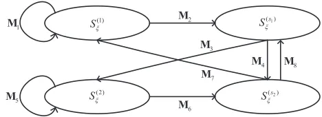
M=
M1 M2 0 0 0 0 M3 M4 0 0 M5 M6 M7 M8 0 0
,
where the matrices Mi (i= 1,2,· · ·,8) describe the
tran-sition probabilities among the states in Sξ, see Fig. 4. It
can be seen that, some blocks in M are zero matrices. That is because the swithover times of the server between the two queues are not ignored. The structure of M will provide conveniences for the following analysis, see Section III-B and Section III-C. The details about the matrices Mi
(i= 1,2, · · ·,8)will be given respectively in the following.
(1) S[
1
M M2
3 M
4 M
5 M
6 M
7 M
8 M
1 ( )s
S[
(2)
[image:8.576.300.534.212.297.2]S[ S[(s2)
FIGURE 4. The schematic diagram of the one-step transitions among the states inSξ.
For making some expressions concise, two notations are introduced firstly. Let
δ(n1, n2) = δn1,n2 1−δn1,n2
,
hΓ(n1, n2)i=
Γ(n1, n2) Γ(n1, n2) Γ(n1, n2) Γ(n1, n2)
,
where Γ is a universal symbol, and it will be replaced by the required symbols in different cases. The meanings and calculation formulas of Γ(n1, n2), Γ(n1, n2), Γ(n1, n2)
andΓ(n1, n2)are presented in Appendix A.
(1) The matrix M1 describes the one-step transitions
a-mong the states in Sξ(1). Within Sξ(1), the state with
φ= (1, i, i)can not transfer to any other states, where
i ∈ {1,2,· · · , Q1}; the state with φ = (1, i, k)can
transfer to the state with φ = (1, i, k+ 1), where
i ∈ {2,3,· · ·, Q1},k ∈ {1,2,· · ·, i−1}. So, M1
has the following structure.
M1=diag M1,1 M1,2 · · · M1,Q1
,
whereM1,1 = 0ς1,ςn = ¯m(Q1−n+ 1) (Q2+ 1), n∈ {0,1,· · ·, Q1}; and
M1,i=
0 (M1,i)1,2 · · · 0
..
. ... . .. ...
0 0 · · · (M1,i)i−1,i
0ς1×ςi 0 · · · 0
,
i∈ {2,3,· · ·, Q1}.(M1,i)k,k+1,i∈ {2,3,· · · , Q1},
are indexed by (l1, l2),(l10, l02)
,(l1, l2)∈L(11,i−k)×
L(1)2 ,(l10, l02)∈L
(1,i−k−1)
1 ×L
(1) 2 , where
(M1,i)k,k+1
(l1,l2),(l01,l02)
=P
(1, i, k+ 1), l01, l02|(1, i, k), l1, l2 .
Giveniandk, consider each(l1, l2)∈L(11,i−k)×L (1)
2 ,
(a) for (l01, l20) ∈ {l1−1, l1,· · · , Q1−1} × {l2,
l2+ 1,· · ·, Q2},
(M1,i)k,k+1
(l1,l2),(l01,l02)
=δ(Q2, l20)hB1(l10 −l1+ 1, l02−l2)iδT
×(Q1, l01+ 1) ;
(b) for the other(l01, l02)∈L1(1,i−k−1)×L (1)
2 ,
(M1,i)k,k+1
(l1,l2),(l01,l02)
=0m¯.
(2) The matrixM2describes the one-step transitions of the
states fromSξ(1) toS(s1)
ξ . Consider the states inS
(1)
ξ ,
only the state withφ = (1, i, i)can enter into S(s1) ξ ,
wherei ∈ {1,2,· · · , Q1}. So,M2has the following
structure.
M2=
M2,1,0 M2,1,1 · · · M2,1,Q1−1
M2,2,0 M2,2,1 · · · M2,2,Q1−1
..
. ... . .. ...
M2,Q1,0 M2,Q1,1 · · · M2,Q1,Q1−1
,
where
M2,1,j =M2,j, j ∈ {0,1,· · · , Q1−1},
M2,i,j= 0Si−1
Q1−1×ςj M2,j
!
, i∈ {2,3,· · · , Q1},
j ∈ {0,1,· · · , Q1−1},
andSk
n = ¯m(Q2+ 1) [n+ (n−1) + (n−2) +· · · +(n−k+ 1)].M2,j,j ∈ {0,1,· · · , Q1−1},
con-sists of matrix blocks which are indexed by (l1, l2), (l01, l02)
,(l1, l2)∈L(11,0)×L (1)
2 ,(l01, l20)∈ L (s1,j)
1 ×
L(2s1), where
(M2,j)(l1,l2),(l0
1,l02)
=P
(s1, j), l01, l20|(1, i, i), l1, l2 .
Givenj, consider each(l1, l2)∈
L(11,0)\ {j}
×L(1)2 ,
for any(l01, l02)∈L(1s1,j)×L (s1)
2 ,
(M2,j)(l1,l2),(l0
1,l02) =0m¯;
consider each(l1, l2)∈ {j} ×L(1)2 ,
(a) for(l01, l20)∈L1(s1,j)× {l2, l2+ 1,· · ·, Q2},
(M2,j)(l1,l2),(l0
1,l02)
=δ(Q2, l20)hR1(l01−l1, l02−l2)iδT(Q1, l01),
(b) for the other(l10, l02)∈L(s1,j)
1 ×L
(s1)
2 ,
(M2,j)(l
1,l2),(l10,l02) =0m¯.
(3) The matrix M3 describes the one-step transitions of
the states fromS(s1) ξ toS
(2)
ξ . In this case, the state with φ= (s1, j)inS
(s1)
ξ may only transfer to the state with φ= (2, j)inSξ(2), wherej ∈ {0,1,· · · , Q1−1}. So, M3has the following structure.
M3=diag M3,0 M3,1 · · · M3,Q1−1
,
where M3,j, j ∈ {0,1,· · ·, Q1−1}, consists of
matrix blocks which are indexed by (l1, l2),(l01, l02)
, (l1, l2)∈L(1s1,j)×L
(s1)
2 ,(l10, l20)∈L (2,j)
1 ×L
(2) 2 , where
(M3,j)(l1,l2),(l0
1,l02) =P
(2, j), l10, l02|(s1, j), l1, l2 .
Givenj, consider each(l1, l2)∈L(1s1,j)× {0}, for any (l01, l02)∈L(21,j)×L(2)2 ,
(M3,j)(l
1,l2),(l10,l02) =0m¯;
consider each(l1, l2)∈L(1s1,j)×
L(2s1)\ {0}
,
(a) for(l0
1, l02)∈ {l1, l1+ 1,· · ·, Q1} × {l2−1, l2, · · · , Q2−1},
(M3,j)(l
1,l2),(l01,l02)
=δ(Q2, l02+ 1)
×
Hj◦B2(l01−l1, l02−l2+ 1)
×δT(Q1, l01),
(b) for the other(l10, l02)∈L(21,j)×L (2)
2 ,
(M3,j)(l1,l2),(l0
1,l02) =0m¯.
(4) The matrixM4describes the one-step transitions of the
states fromS(s1) ξ toS
(s2)
ξ . Any state inS
(s1)
ξ may enter
intoS(s2)
ξ . So,M4has the following structure.
M4= M4,0 M4,1 M4,2 · · · M4,Q1−1
T
,
where M4,j, j ∈ {0,1,· · ·, Q1−1}, consists of
matrix blocks which are indexed by (l1, l2),(l01, l02)
, (l1, l2)∈L(1s1,j)×L
(s1)
2 ,(l01, l20)∈L (s2)
1 ×L
(s2)
2 , where
(M4,j)(l
1,l2),(l01,l02) =P
s2, l10, l 0
2|(s1, j), l1, l2 .
Givenj, consider each(l1, l2)∈L(1s1,j)× {0},
(a) for(l0
1, l02)∈ {l1, l1+ 1,· · · , Q1} ×L(2s2)
(M4,j)(l 1,l2),(l01,l
0
2)
=δ(Q2, l20)hR2(l01−l1, l02)iδ
T(Q
1, l10),
(b) for the other(l0
1, l02)∈L (s2)
1 ×L
(s2)
2 ,
(M4,j)(l 1,l2),(l01,l
0
2) =
0m¯;
consider each(l1, l2)∈L(1s1,j)×
L(2s1)\ {0}
(a) for(l01, l02)∈ {l1, l1+ 1,· · ·, Q1} × {l2, l2+ 1, · · ·, Q2},
(M4,j)(l1,l2),(l0
1,l02)
=
l01−l1
X
i1=0 l02−l2
X
i2=0
δ(Q2, l2+i2)
B2◦Hj(i1, i2)
×δT(Q1, l1+i1)δ(Q2, l02) × hR2(l01−l1−i1, l20 −l2−i2)i
×δT(Q1, l10),
(b) for the other(l01, l02)∈L(1s2)×L (s2)
2
(M4,j)(l
1,l2),(l10,l02) =0m¯.
(5) The matrix M5 describes the one-step transitions
a-mong the states in Sξ(2). Within Sξ(2), the state with
φ= (2, j)may only transfer to the state with the same
φ= (2, j), wherej∈ {0,1,· · ·, Q1−1}. So,M5has
the following structure.
M5=diag M5,0 M5,1 · · · M5,Q1−1
,
where M5,j, j ∈ {0,1,· · · , Q1−1}, consists of
matrix blocks which are indexed by (l1, l2),(l01, l20)
, (l1, l2),(l01, l20)∈L
(2,j)
1 ×L
(2) 2 , where
(M5,j)(l1,l2),(l0
1,l02) =P
(2, j), l10, l02|(2, j), l1, l2 .
Givenj, consider each(l1, l2)∈L(21,j)× {0}, for any (l01, l02)∈L(21,j)×L(2)2 ,
(M5,j)(l1,l2),(l0
1,l02) =
0m¯;
consider each(l1, l2)∈L(21,j)×
L(2)2 \ {0}
,
(a) for(l01, l02)∈ {l1, l1+ 1,· · ·, Q1} × {l2−1, l2, · · ·, Q2−1},
(M5,j)(l
1,l2),(l01,l02)
=δ(Q2, l02+ 1)
×
Hj◦B2(l10 −l1, l02−l2+ 1)
×δT(Q1, l01),
(b) for the other(l01, l02)∈L (2,j)
1 ×L
(2)
2 ,
(M5,j)(l
1,l2),(l10,l02) =0m¯.
(6) The matrixM6describes the one-step transitions of the
states fromSξ(2)toS(s2)
ξ . Any state inS
(2)
ξ may enter
intoS(s2)
ξ . So,M6has the following structure.
M6= M6,0 M6,1 M6,2 · · · M6,Q1−1
T
,
where M6,j, j ∈ {0,1,· · · , Q1−1}, consists of
matrix blocks which are indexed by (l1, l2),(l01, l20)
, (l1, l2)∈L(21,j)×L
(2)
2 ,(l01, l02)∈L (s2)
1 ×L
(s2)
2 , where
(M6,j)(l1,l2),(l0
1,l02) =P
s2, l01, l02|(2, j), l1, l2 .
Givenj, consider each(l1, l2)∈L(21,j)× {0},
(a) for(l01, l02)∈ {l1, l1+ 1,· · · , Q1} ×L(2s2),
(M6,j)(l1,l2),(l01,l
0
2)
=δ(Q2, l20)hR2(l01−l1, l02)iδ
T(Q
1, l10),
(b) for the other(l10, l02)∈L(1s2)×L (s2)
2 ,
(M6,j)(l 1,l2),(l01,l
0
2) =
0m¯;
consider each(l1, l2)∈L(21,j)×
L(2)2 \ {0}
,
(a) for(l01, l02)∈ {l1, l1+ 1,· · ·, Q1} × {l2, l2+ 1, · · · , Q2},
(M6,j)(l1,l2),(l0
1,l02)
=
l01−l1
X
i1=0 l02−l2
X
i2=0
δ(Q2, l2+i2)
B2◦Hj(i1, i2)
×δT(Q1, l1+i1)δ(Q2, l02) × hR2(l01−l1−i1, l20 −l2−i2)i
×δT(Q1, l01),
(b) for the other(l10, l02)∈L (s2)
1 ×L
(s2)
2 ,
(M6,j)(l1,l2),(l0
1,l02) =0m¯.
(7) The matrix M7 describes the one-step transitions of
the states from S(s2) ξ to S
(1)
ξ . Only the state with φ = (1, i,1) in S(1)ξ can be reached, where i ∈ {1,2,· · ·, Q1}. So,M7has the following structure.
M7= M7,1,1 M7,1,2 M7,1,3 · · · M7,1,Q1
,
where
M7,1,1=M7,1,
M7,1,i=
M7,i 0ς0×SiQ−11
, i∈ {2,3,· · ·, Q1}.
M7,i,i ∈ {1,2,· · ·, Q1}, consists of matrix blocks
which are indexed by (l1, l2), (l01, l02)
, (l1, l2) ∈
L(1s2)×L (s2)
2 ,(l01, l02)∈L (1,i−1)
1 ×L
(1) 2 , where
(M7,i)(l 1,l2),(l01,l
0
2) =
P
(1, i,1), l01, l20|s2, l1, l2 .
Given i, i ∈ {1,2,· · ·, Q1}, consider (l1, l2) ∈
L(1s2)\ {i}
×L(s2)
2 , for any(l10, l02) ∈ L (1,i−1)
1 ×
L(1)2 ,
(M7,i)(l1,l2),(l0
1,l02) =0m¯;
consider(l1, l2)∈ {i} ×L(2s2),
(a) for(l01, l02)∈L1(1,i−1)× {l2, l2+ 1,· · ·, Q2},
(M7,i)(l 1,l2),(l01,l
0
2)
=δ(Q2, l02)hB1(l10 −l1+ 1, l20 −l2)i
(b) for the other(l01, l02)∈L(11,i−1)×L(1)2 ,
(M7,i)(l 1,l2),(l01,l
0
2) =
0m¯.
(8) The matrix M8 describes the one-step transitions of
the states from S(s2) ξ to S
(s1)
ξ . Only the state with φ = (s2,0)inS
(s1)
ξ can be reached. So, M8 has the
following structure.
M8=
M8,0 0ς
0×SQQ1−1 1
,
whereM8,0 consists of matrix blocks which are
in-dexed by (l1, l2),(l01, l02)
,(l1, l2)∈ L(1s2)×L (s2)
2 ,
(l01, l02)∈L(1s1,0)×L (s1)
2 , where
(M8,0)(l1,l2),(l0
1,l20) =P
(s1,0), l01, l02|s2, l1, l2 .
Consider (l1, l2) ∈
L(1s2)\ {0}
× L(2s2), for any
(l01, l02)∈L(1s1,0)×L (s1)
2 ,
(M8,0)(l1,l2),(l0
1,l02) =0m¯;
consider(l1, l2)∈ {0} ×L(2s2),
(a) for(l01, l20)∈L1(s1,0)× {l2, l2+ 1,· · · , Q2},
(M8,0)(l1,l2),(l0
1,l20)
=δ(Q2, l02)hR1(l10, l02−l2)iδT(Q1, l01),
(b) for the other(l01, l02)∈L(1s1,0)×L (s1)
2 ,
(M8,0)(l1,l2),(l0
1,l02) =0m¯.
The states of the Markov chain
ξn;n∈N+ satisfy the
properties.
Property 1: For the zero state (s2,0,0, v1, v2),v1 ∈ M1,
v2 ∈M2, it can be reached from any state inSξ. The reason
is that the BMAP-1 and the BMAP-2 are independent;D(1)
andD(2)are irreducible;D(1)
0 andD
(2)
0 are stable.
Property 2:There is a state subspace denoted bySˆξ, which
consists of the states(s2,0,0, v1, v2),v1 ∈ M1,v2 ∈ M2,
and the states which can be reached from any of the states (s2,0,0, v1, v2),v1 ∈ M1,v2 ∈ M2. So,Sˆξ is irreducible
and aperiodic. From this and Property 1, it follows that the Markov chain
ξn;n∈N+ has the stationary distribution
in its state spaceSξ.
B. THE JOINT QUEUE LENGTH STATIONARY DISTRIBUTION AT QUEUE 1 POLLING EPOCHS
Consider the event that a switchover of the server from queue 2 to queue 1 just terminates. Let Tn0 n∈N+
be the instant when this event occurs at the n-th time. The state of the cyclic polling model at T0
n is denoted by ξ0(Tn0) = L1(Tn0), L2(Tn0), V1(Tn0), V2(Tn0)
, whereLι(Tn0)
and Vι(Tn0) represent the same meanings as the ones
cor-responding to ξ(Tn). ξ0(Tn0) is briefly denoted by ξ0n = L01,n, L02,n, V10,n, V20,n
. The discrete-time stochastic pro-cessξn0;n∈N+ is constructed, and it is a homogeneous
Markov chain on the state spaceSξ0 =L(s2)
1 ×L
(s2)
2 ×M1×
M2. Based on the one-step transition probability matrixM
of the Markov chain
ξn;n∈N+ , the one-step transition
probability matrix W of the Markov chain
ξ0n;n∈N+ can be given by
W= "
M7,1+
Q1
X
i=2 M7,i
i
Y
k=2
(M1,i)k−1,k
#
× Q1−1
X
j=0 M2,j
"
M4,j+M3,j
∞ X
k=0 Mk5,j
!
M6,j
#
+M8,0 "
M4,0+M3,0 ∞ X
k=0 Mk5,0
!
M6,0 #
. (8)
Based on Property 1 and Property 2, it can be proved by contradiction that the Markov chain ξn0;n∈N+ has the stationary distribution in Sξ0. Let the probability vector ω denote the stationary distribution ofξ0n;n∈N+ , i.e.
ω=ω(l1,l2): (l1, l2)∈L
(s2)
1 ×L
(s2)
2
,
where
ω(l1,l2)=
ω(l1,l2)
(v1,v2): (v1, v2)∈M1×M2
,
ω(l1,l2)
(v1,v2)= limn→∞P
ξn0 = (l1, l2, v1, v2) .
ω is also the joint queue length stationary distribution at queue 1 polling epochs, where ω(l1,l2)
(v1,v2) represents
the stationary probability that, at queue 1 polling epochs, the length of queue 1 isl1, the length of queue 2 isl2, the phase
of the BMAP-1 isv1, and the phase of the BMAP-2 isv2.ω
satisfies the following relations,
(
ωW=ω,
ωe= 1. (9)
Based on the GTH algorithm [36], ω can be obtained by solving the system of linear equations (9).
C. THE JOINT QUEUE LENGTH STATIONARY DISTRIBUTION AT QUEUE 2 POLLING EPOCHS
Consider the event that a switchover of the server from queue 1 to queue 2 just terminates. LetTn00 n∈N+be the instant when this event occurs at then-th time. The state of the cyclic polling model atTn00is denoted by
ξ00(Tn00) = Φ(Tn00), L1(Tn00), L2(Tn00), V1(Tn00), V2(Tn00)
,
whereΦ(Tn00),Lι(Tn00)andVι(Tn00)represent the same
mean-ings as the ones corresponding to ξ(Tn).ξ00(Tn00) is briefly
denoted byξ00n= Φ00n, L001,n, L002,n, V100,n, V200,n
. The discrete-time stochastic processξn00;n∈N+ is constructed, and it
is a homogeneous Markov chain on the state spaceS(s1) ξ .
Based on Property 1 and Property 2, it can be proved by contradiction that the Markov chain
ξn00;n∈N+ has the stationary distribution inS(s1)
ξ . Let the probability vectorθ
denote the stationary distribution of
ξ00n;n∈N+ .
where for eachj∈ {0,1,· · ·, Q1−1},
θ(s1,j)=θ(s1,j)
(l1,l2): (l1, l2)∈L
(s1,j)
1 ×L
(s1)
2
,
θ(s1,j)
(l1,l2)=
θ(s1,j)
(l1,l2)
(v1,v2)
: (v1, v2)∈M1×M2
,
θ(s1,j)
(l1,l2)
(v1,v2)
= lim
n→∞P n
ξn00= (s1, j), l1, l2, v1, v2 o
.
There is the following relationship betweenθandω.
θ(s1,0)=ω
( "
M7,1+
Q1
X
i=2 M7,i
i
Y
k=2
(M1,i)k−1,k
#
M2,0
+M8,0 )
, (10)
θ(s1,j)=ω
"
M7,1+
Q1
X
i=2 M7,i
i
Y
k=2
(M1,i)k−1,k
#
×M2,j, j ∈ {1,2,· · · , Q1−1}. (11)
Let the probability vectorηdenote the joint queue length stationary distribution at queue 2 polling epochs.
η= η(l1,l2): (l1, l2)∈L1×L2
,
whereL1={0,1,· · ·, Q1},L2={0,1,· · ·, Q2},
η(l1,l2)=
η(l1,l2)
(v1,v2): (v1, v2)∈M1×M2
,
η(l1,l2)
(v1,v2)= l1
X
j=0
θ(s1,j)
(l1,l2)
(v1,v2)
. (12)
η(l1,l2)
(v1,v2)represents the stationary probability that, at
queue 2 polling epochs, the length of queue 1 isl1, the length
of queue 2 isl2, the phase of the BMAP-1 isv1, and the phase
of the BMAP-2 isv2.
IV. THE JOINT QUEUE LENGTH STATIONARY DISTRIBUTION AT ARBITRARY TIME
From Property 2, the Markov chain
ξn;n∈N+ has the
stationary distribution in the state spaceSξ. Let the stationary
distribution be denoted by the probability vector π, which satisfies the following relations,
πM=π, πe= 1. (13)
πcan be divided into four parts, i.e.
π= π(1) π(s1) π(2) πs2.
(1)
π(1) = π(1,1,1) π(1,2,1) π(1,2,2) · · ·
π(1,Q1,1) π(1,Q1,2) · · · π(1,Q1,Q1),
where fori∈ {1,2,· · · , Q1},k∈ {1,2,· · ·, i},
π(1,i,k)=π(1(l,i,k)
1,l2) : (l1, l2)∈L
(1,i−k)
1 ×L
(1) 2
,
π((1l,i,k)
1,l2) =
π(1(l,i,k)
1,l2)
(v1,v2)
: (v1, v2)∈M1×M2
,
π((1l,i,k)
1,l2)
(v1,v2)
= lim
n→∞P n
ξn= (1, i, k), l1, l2, v1, v2 o
;
(2)
π(s1)= π(s1,0) π(s1,1) · · · π(s1,Q1−1),
where forj∈ {0,1,· · · , Q1−1},
π(s1,j)=
π(s1,j)
(l1,l2): (l1, l2)∈L
(s1,j)
1 ×L
(s1)
2
,
π(s1,j)
(l1,l2)=
π(s1,j)
(l1,l2)
(v1,v2)
: (v1, v2)∈M1×M2
,
π(s1,j)
(l1,l2)
(v1,v2)
= lim
n→∞P n
ξn= (s1, j), l1, l2, v1, v2 o
;
(3)
π(2) = π(2,0) π(2,1) · · · π(2,Q1−1),
where forj∈ {0,1,· · · , Q1−1},
π(2,j)=π(2(l,j)
1,l2): (l1, l2)∈L
(2,j)
1 ×L
(2) 2
,
π((2l,j)
1,l2)=
π(2(l,j)
1,l2)
(v1,v2)
: (v1, v2)∈M1×M2
,
π((2l,j)
1,l2)
(v1,v2)
= lim
n→∞P n
ξn= (2, j), l1, l2, v1, v2 o
;
(4)
πs2 =
πs2
(l1,l2): (l1, l2)∈L
(s2)
1 ×L
(s2)
2
,
where
πs2
(l1,l2)=
πs2
(l1,l2)
(v1,v2)
: (v1, v2)∈M1×M2
,
πs2
(l1,l2)
(v1,v2)
= lim
n→∞P
ξn= (s2, l1, l2, v1, v2) .
Based on the relations in (13) and the structures ofMand π, there are the following relations.
π(1,i,1)=πs2M
7,i, i∈ {1,2,· · · , Q1}, (14)
π(1,i,k)=π(1,i,k−1)(M1,i)k−1,k, i∈ {2,3,· · · , Q1},
k∈ {2,3,· · ·, i}; (15)
π(s1,0)=πs2M
8,0+
Q1
X
i=1
π(1,i,i)M2,0, (16)
π(s1,j)= Q1
X
i=1
π(2,j)=π(s1,j)M
3,j(I−M5,j)
−1
,
j∈ {0,1,· · ·, Q1−1}. (18)
From (14), (15), (16), (17) and (18), it can be seen that if πs2 is given, the other parts ofπcan be calculated directly.
There is a constantc(0< c <∞), such thatπs2 =cω. So,
the stationary distributionπcan be obtained as the following way. First, setπs2 = ω; then from the relations (14), (15),
(16), (17) and (18), the vector π is calculated; finally, the stationary distribution is obtained by normalizingπ.
Let ˜
Sξ = ˜S
(1)
ξ
[˜
S(s1) ξ
[˜
Sξ(2)[S˜(s2) ξ ,
where
˜
Sξ(1)=
Q1 [ i=1 i [ k=1
{(1, i, k)} ×L(11,i−k)×L (1)
2 ,
˜
S(s1)
ξ =
Q1−1
[
j=0
{(s1, j)} ×L(1s1,j)×L (s1)
2 ,
˜
Sξ(2)=
Q1−1
[
j=0
{(2, j)} ×L(21,j)×L (2)
2 ,
˜
S(s2)
ξ ={s2} ×L(1s2)×L (s2)
2 .
From
ξn;n∈N+ , a Markov renewal process
ξn, Tn;n∈N+ can be constructed. The mean time
be-tween two successive renewals of the Markov renewal process ξn, Tn;n∈N+ is denoted by τ, and it can be
calculated by τ = Q1 X i=1 i X k=1
Q1−1
X
l1=i−k Q2
X
l2=0
π((1l,i,k)
1,l2)m
(1,i,k) (l1,l2)
+
Q1−1
X
j=0
Q1
X
l1=j Q2
X
l2=0
π(s1,j)
(l1,l2)m
(s1,j)
(l1,l2)
+
Q1−1
X
j=0
Q1
X
l1=j Q2−1
X
l2=0
π(2(l,j)
1,l2)m
(2,j) (l1,l2)
+
Q1
X
l1=0 Q2
X
l2=0
πs2
(l1,l2)m s2
(l1,l2). (19)
(1) Given (1, i, k), l1, l2
∈ S˜(1)
ξ , m
(1,i,k)
(l1,l2) is a m¯
-dimensional column vector,
m(1(l,i,k)
1,l2)
=
m(1(l,i,k)
1,l2)
(v1,v2)
: (v1, v2)∈M1×M2 T
,
where the(v1, v2)-th element denotes the mean time
from a renewal with the state (1, i, k), l1, l2, v1, v2
to the next renewal. For any (1, i, k), l1, l2∈S˜ (1)
ξ ,
m(1(l,i,k)
1,l2)=
(
b1em¯, fork < i,
r1em¯, fork=i.
(2) Given (s1, j), l1, l2
∈ S˜(s1)
ξ , m
(s1,j)
(l1,l2) is a m¯
-dimensional column vector,
m(s1,j)
(l1,l2)
=
m(s1,j)
(l1,l2)
(v1,v2)
: (v1, v2)∈M1×M2 T
,
where the (v1, v2)-th element denotes the mean time
from a renewal with the state (s1, j), l1, l2, v1, v2
to the next renewal. Consider each (s1, j), l1, l2
∈
˜
S(s1) ξ ,
(a) forl2= 0,
m(s1,j)
(l1,l2)=r2em¯;
(b) forl26= 0,
m(s1,j)
(l1,l2)
= Z ∞ t=0 1− Z t x=0
[1−Hj(x)]dB2(x)
− Z t
x=0
[1−B2(x)]dHj(x)
×R2(t−x)
dtem¯
=
β2 γjImB2 −B2 −1
emB2−α2R−21emR2
×hγjβ2 γjImB2 −B2
−1 emB2
i em¯.
(3) Given (2, j), l1, l2 ∈ S˜ (2)
ξ , m
(2,j)
(l1,l2) is a m¯
-dimensional column vector,
m(2(l,j)
1,l2)
=
m(2(l,j)
1,l2)
(v1,v2)
: (v1, v2)∈M1×M2 T
,
where the (v1, v2)-th element denotes the mean time
from a renewal with the state (2, j), l1, l2, v1, v2
to the next renewal. Consider each (2, j), l1, l2
∈
˜
Sξ(2),
(a) forl2= 0,
m(2(l,j)
1,l2)=r2em¯;
(b) forl26= 0,
m(2(l,j)
1,l2)
= Z ∞ t=0 1− Z t x=0
[1−Hj(x)]dB2(x)
− Z t
x=0
[1−B2(x)]dHj(x)
×R2(t−x)
dtem¯
=
β2 γjImB2 −B2
−1
emB2−α2R
−1 2 emR2
×hγjβ2 γjImB2 −B2 −1
emB2
(4) Given(s2, l1, l2)∈S˜ (s2) ξ ,m
s2
(l1,l2)is am¯-dimensional
column vector,
ms2
(l1,l2)
=
ms2
(l1,l2)
(v1,v2)
: (v1, v2)∈M1×M2 T
,
where the(v1, v2)-th element denotes the mean time
from a renewal with the state(s2, l1, l2, v1, v2)to the
next renewal. Consider each(s2, l1, l2)∈S˜ (s2) ξ ,
(a) forl1= 0,
ms2
(l1,l2)=r1em¯;
(b) forl16= 0,
ms2
(l1,l2)=b1em¯.
Let χ(t) = L1(t), L2(t), V1(t), V2(t)
denote the state of the cyclic polling model at arbitrary timet(t≥0), whereLι(t)andVι(t) represent the same meanings as the
ones corresponding toξ(Tn)in Section III-A, Lι(t) ∈ Lι, Vι(t)∈ Mι. Consider the stochastic process{χ(t) ;t≥0}
on the state spaceS = L1×L2×M1×M2, and assume
that for any sample path t → χ(t), it is right continuous and has left-hand limit. According to the definition 10.6.1 of [31],{χ(t) ;t≥0} is a semi-regenerative process with the corresponding Markov renewal process
ξn, Tn;n∈N+ .
For(φ, l1, l2)∈S˜ξ,(l01, l02)∈L1×L2, define the matrix K (φ, l1, l2),(l01, l20), t
,
K((φ, l1, l2),(l01, l 0 2), t)
= K(v
1,v2),(v01,v20) (φ, l1, l2),(l
0 1, l
0 2), t
: (v1, v2),(v10, v02)∈M1×M2 !
,
where the (v1, v2),(v10, v20)
-th element denotes the fol-lowing conditional probability,
K(v
1,v2),(v10,v02) (φ, l1, l2),(l
0 1, l02), t
=PnL1(t) =l10, L2(t) =l20, V1(t) =v10, V2(t) =v20,
t < T |Φ(0) =φ, L1(0) =l1, L2(0) =l2,
V1(0) =v1, V2(0) =v2 o
,
T is a random variable denoting the time from the renewal with the state (φ, l1, l2, v1, v2) to the next renewal of the
Markov renewal process{ξn, Tn;n∈ N+ . The expression
for each K((φ, l1, l2),(l01, l20), t)is given in Appendix B.
And
Kφ
(l1,l2),(l10,l
0
2)
= Z ∞
t=0
K (φ, l1, l2),(l01, l 0 2), t
dt <∞,
where the calculation formula of eachKφ
(l1,l2),(l01,l
0
2)
is also
given in Appendix B.
Based on Property 1 and Property 2,
ξn, Tn;n∈N+
can enter into the state subspace Sˆξ eventually and is an
irreducible aperiodic recurrent process in Sˆξ. According to
Theorem 10.6.12 of [31], {χ(t) ;t≥0} has the stationary distribution denoted byp, ast→ ∞.
p=p(l0
1,l
0
2) : (
l10, l02)∈L1×L2
,
where
p(l0
1,l02) =
p(l0
1,l02)
(v0
1,v
0
2)
: (v10, v02)∈M1×M2
,
p(l0
1,l02)
(v0
1,v02)
= lim
t→∞P{χ(t) = (l 0 1, l
0 2, v
0 1, v
0 2)}.
pis also the joint queue length stationary distribution at arbi-trary time, where p(l0
1,l02)
(v0
1,v
0
2)
represents the stationary
probability that, at arbitrary time, the length of queue 1 isl01, the length of queue 2 isl20, the phase of the BMAP-1 isv01, and the phase of the BMAP-2 isv20.pcan be calculated as follows. Given(l10, l02)∈L1×L2,
p(l0
1,l
0
2) =
1
τ
X
(φ,l1,l2)∈Sξ˜
πφ(l
1,l2)K φ
(l1,l2),(l01,l20) .
(1) Forl01= 0,l02= 0,
p(0,0)= 1
τ
( Q1
X
i=1
π(0(1,i,i,0))K(0(1,,i,i0),)(0,0)
+π(s1,0)
(0,0) K (s1,0)
(0,0),(0,0)+π (2,0) (0,0)K
(2,0) (0,0),(0,0)
+πs2
(0,0)K
s2
(0,0),(0,0) )
; (20)
(2) Forl01= 0,l02∈ {1,2,· · · , Q2},
p(0,l0
2) =
1
τ
Q1
X
i=1
l02
X
l2=0
π(0(1,i,i,l )
2)K
(1,i,i) (0,l2),(0,l02)
+
l02
X
l2=0
π(s1,0)
(0,l2)K
(s1,0)
(0,l2),(0,l02)
+ ∆l0
2
X
l2=0
π(2(0,l,0)
2)K
(2,0) (0,l2),(0,l02)
+
l0
2
X
l2=0
πs2
(0,l2)K s2
(0,l2),(0,l02)
, (21)
where∆l0
2 =δQ2,l02(Q2−1) +
1−δQ2,l0
2
(3) Forl10 ∈ {1,2,· · ·, Q1},l02= 0,
p(l0
1,0)
= 1
τ
∆l0
1
X
l1=1 Q1
X
i=2
min{l1,i−1}
X
η=1
π(1(l,i,i−η)
1,0) K
(1,i,i−η) (l1,0),(l01,0)
+
Q1
X
i=1 ∆l0
1
X
l1=0
π((1l,i,i)
1,0)K
(1,i,i) (l1,0),(l01,0)
+
Q1−1
X
j=0
l0
1
X
l1=j
π(s1,j)
(l1,0)K
(s1,j)
(l1,0),(l01,0)
+
Q1−1
X
j=0
l01
X
l1=j
π(2(l,j)
1,0)K
(2,j) (l1,0),(l01,0)
+
l01
X
l1=0
πs2
(l1,0)K s2
(l1,0),(l01,0)
, (22)
where∆l0
1 =δQ1,l01(Q1−1) +
1−δQ1,l0
1
l01; (4) Forl10 ∈ {1,2,· · ·, Q1},l02∈ {1,2,· · ·, Q2},
p(l0
1,l02)
= 1
τ
∆l0
1
X
l1=1 Q1
X
i=2
min{l1,i−1}
X
η=1
l02
X
l2=0
π(1(l,i,i−η)
1,l2) K
(1,i,i−η) (l1,l2),(l01,l02)
+
Q1
X
i=1 ∆l0
1
X
l1=0 l02
X
l2=0
π((1l,i,i)
1,l2)K
(1,i,i) (l1,l2),(l01,l02)
+
Q1−1
X
j=0
l01
X
l1=j l02
X
l2=0
π(s1,j)
(l1,l2)K
(s1,j)
(l1,l2),(l01,l02)
+
Q1−1
X
j=0
l01
X
l1=j
∆l0
2
X
l2=0
π(2(l,j)
1,l2)K
(2,j) (l1,l2),(l01,l02)
+
l01
X
l1=0 l02
X
l2=0
πs2
(l1,l2)K s2
(l1,l2),(l01,l
0 2) . (23)
Remark 1:The cyclic polling model presented in this paper is consistent with the one presented by [13], except that the buffer sizes are finite. In [13], the stability condition of the cyclic polling model with infinite-buffer queues was analyzed. Under this stability condition, the joint queue length stationary distributions of the cyclic polling model with infinite-buffer queues can be obtained asymptotically, by increasing the buffer sizes of the corresponding cyclic polling model with finite-buffer queues.
V. CUSTOMER BLOCKING PROBABILITIES AND WAITING TIMES
Let k ∈ N+,n1 ∈ {0,1,· · ·, Q1},n2 ∈ {0,1,· · · , Q2}.
Consider the event that, at arbitrary time the lengths of queue 1 and queue 2 are n1 and n2 respectively, and at
the same time there is a batch arrival of size k in queue 1. The probability that the event occurs can be expressed
as p(n1,n2)
kD(1)k ⊗Im(2)
λ1 em¯. When the size of the batch
arriving at queue 1 is k, if the length of queue 1 is n1 (k > Q1−n1), the probability that any customer in this
batch is blocked is k−(Q1−n1)
k . So, the probability that any
customer arriving at queue 1 is blocked can be expressed as the following.
P1,BL
=
Q1
X
n1=0 Q2
X
n2=0
p(n1,n2)
×
∞ X
k=Q1−n1+1
kD(1)k ⊗Im(2)
λ1
×k−(Q1−n1)
k em¯
=
Q1
X
n1=0 Q2
X
n2=0
p(n1,n2)
×
∞ X
k=Q1−n1+1
λ−11D(1)k ⊗Im(2)
[k−(Q1−n1)]em¯.
(24)
Consider the event that, at arbitrary time the lengths of queue 1 and queue 2 are n1 and n2 respectively, and at
the same time there is a batch arrival of size k in queue 2. The probability that the event occurs can be expressed
as p(n1,n2) kI
m(1)⊗D (2) k
λ2 em¯. When the size of the batch
arriving at queue 2 is k, if the length of queue 2 is n2 (k > Q2−n2), the probability that any customer in this
batch is blocked is k−(Q2−n2)
k . So, the probability that any
customer arriving at queue 2 is blocked can be expressed as the following.
P2,BL
=
Q1
X
n1=0 Q2
X
n2=0
p(n1,n2)
×
∞ X
k=Q2−n2+1
kIm(1)⊗D
(2)
k
λ2
×k−(Q2−n2)
k em¯
=
Q1
X
n1=0 Q2
X
n2=0
p(n1,n2)
×
∞ X
k=Q2−n2+1
λ−21Im(1)⊗D
(1)
k
[k−(Q2−n2)]em¯.
(25)
Let W¯1 and W¯2 represent the mean waiting times of