www.geosci-model-dev.net/7/821/2014/ doi:10.5194/gmd-7-821-2014
© Author(s) 2014. CC Attribution 3.0 License.
Geoscientific
Model Development
Effects of vegetation structure on biomass accumulation in a
Balanced Optimality Structure Vegetation Model (BOSVM v1.0)
Z. Yin1, S. C. Dekker2, B. J. J. M. van den Hurk1,3, and H. A. Dijkstra1
1Institute for Marine and Atmospheric research Utrecht, Utrecht University, Utrecht, the Netherlands 2Copernicus Institute of Sustainable Development, Utrecht University, Utrecht, the Netherlands 3Royal Netherlands Meteorological Institute, De Bilt, the Netherlands
Correspondence to: Z. Yin ([email protected])
Received: 18 July 2013 – Published in Geosci. Model Dev. Discuss.: 9 September 2013 Revised: 3 February 2014 – Accepted: 4 March 2014 – Published: 12 May 2014
Abstract. A myriad of interactions exist between vegetation
and local climate for arid and semi-arid regions. Vegetation function, structure and individual behavior have large im-pacts on carbon–water–energy balances, which consequently influence local climate variability that, in turn, feeds back to the vegetation. In this study, a conceptual vegetation struc-ture scheme is formulated and tested in the new Balanced Optimality Structure Vegetation Model (BOSVM) to explore the importance of vegetation structure and vegetation adap-tation to water stress on equilibrium biomass states. Surface energy, water and carbon fluxes are simulated for a range of vegetation structures across a precipitation gradient in West Africa and optimal vegetation structures that maximize biomass for each precipitation regime are determined. Two different strategies of vegetation adaptation to water stress are included. Under dry conditions vegetation tries to maxi-mize the water use efficiency and leaf area index as it tries to maximize carbon gain. However, a negative feedback mech-anism in the vegetation–soil water system is found as the vegetation also tries to minimize its cover to optimize the surrounding bare ground area from which water can be ex-tracted, thereby forming patches of vertical vegetation. Un-der larger precipitation, a positive feedback mechanism is found in which vegetation tries to maximize its cover as it then can reduce water loss from bare soil while having maxi-mum carbon gain due to a large leaf area index. The competi-tion between vegetacompeti-tion and bare soil determines a transicompeti-tion between a “survival” state to a “growing” state.
1 Introduction
Vegetation has a significant impact on the regional climate at different spatial and temporal scales through interactions with the atmosphere, the hydrological cycle and the surface energy balance (Bonan, 2008; Dekker et al., 2010). Posi-tive and negaPosi-tive vegetation–climate feedbacks can affect the local climate variability, particularly in arid and semi-arid regions, owing to the complex vegetation–atmosphere interactions and strong gradients in climate regimes (En-tekhabi et al., 1992; Koster et al., 2004; Dekker et al., 2007; Seneviratne et al., 2010). Vegetation feedbacks mitigate sur-face warming by transpiration, but simultaneously can in-crease the surface energy absorption by reduction of the sur-face albedo, affecting the resilience to drought (Bonan, 2008; Teuling et al., 2010).
In arid and semi-arid areas, water availability is a pri-mary factor for photosynthesis and vegetation development (Seneviratne et al., 2010). In a model experiment, Koster et al. (2004) revealed that soil moisture and precipitation are strongly coupled in water transition zones, including the Western Africa monsoon area. This strong interaction points at a potentially strong role of vegetation–climate interactions in this region. Observations show a good correspondence between maximum vegetation cover and annual mean pre-cipitation (Sankaran et al., 2005; Hirota et al., 2011; Guan et al., 2012). However, for a given precipitation amount the observed cover fraction of woody vegetation varies signifi-cantly. One factor that may play a role here is the vegetation response to fire (Sankaran et al., 2005; Higgins et al., 2010; Hirota et al., 2011; Staver et al., 2011), which will lead to a fast replacement of woody vegetation by grass. This can explain the strong variability of woody vegetation cover in so-called “alternative stable states” (Hirota et al., 2011). Bau-dena et al. (2010) showed how the co-existent regimes of tree and grass species depend on the chosen parameterization op-tions in their conceptual model, pointing at the need for a de-tailed understanding of the underlying biophysical processes. Recently, many studies focus on how precipitation in-fluences vegetation patterns through processes of water re-distribution, such as positive feedbacks due to infiltration (Rietkerk et al., 2002), shading (Baudena and Provenzale, 2008) and topography (Klausmeier, 1999). In these studies transpiration, which is the crucial process in water, carbon and energy balances, is not explicitly modeled. In these con-ceptual models, the transpiration rate simply has a positive relation with biomass density, vegetation fraction or soil wa-ter stress. However, the ability of these conceptual models to describe vegetation dynamics and feedbacks to specific cli-mate is generally limited by their degree to which mechanis-tic processes are included and energy or mass balance clo-sure is satisfied. In addition, different strategies of vegetation response to drought (Calvet, 2000; Calvet et al., 2004) will also influence vegetation fraction and biomass significantly. On the other hand, these conceptual models are tested under simulated precipitation gradient. In fact, across the precipita-tion gradient, other climate variables (radiaprecipita-tion, air humidity, wind speed, soil, etc.) also vary and influence vegetation pro-cesses (Dardel et al., 2014).
In the interaction between vegetation and the coupled carbon–water–energy balances, spatial structure of vegeta-tion plays an important role in transpiravegeta-tion on multiple timescales (e.g., Konings et al., 2011). Within a given set of climate conditions, a large variation of water uptake abil-ity and CO2 assimilation rate exists, controlled by vegeta-tion structure characteristics such as root biomass, leaf area index (LAI) and leaf cover (fc). LAI affects the potential transpiration rate of plants and changes the surface albedo, which controls the solar energy absorption of the land sur-face.fc plays a key role in the vegetation-bare soil compe-tition for water and energy. In water-limited regimes, bare
ground evaporation will reduce the available water needed for photosynthesis, directly affecting biomass accumulation. In addition, the shoot-root distribution of vegetation deter-mines the balance between water uptake and carbon gain.
Both LAI and fc increase as biomass is accumulated. However, for a given leaf biomass, different spatial structures of vegetation can be generated. High LAI/fc values imply an ecosystem developing a vertical structure (e.g., individ-ual trees or patches of dense grasses), while low LAI/fcis representative for horizontally oriented vegetation structures (e.g., grassland or rainforest).
Simultaneously, different strategies exist on regulating stomata response to water stress. Calvet (2000) and Calvet et al. (2004) identified two distinct strategies (drought avoid-ing and drought tolerant), which affect the response of vege-tation to shorter or longer dry periods. Drought tolerant (“of-fensive”) species tend to maximize water use in dry condi-tions, rapidly making benefit of precipitation events in a dry climate. Drought avoiding (“defensive”) strategy leads to a more conservative response to moisture anomalies, aiming at preserving water for times of scarcity.
In this study, our primary objective is to formulate a new vegetation model that considers the effect of spatial struc-ture and adaption to local climate via interactions between the carbon–water–energy cycles. Meanwhile, the new model must be easily linked to existing climate model for further vegetation–land–atmosphere interaction studies.
et al., 2000). In a next study, we will try to enhance our knowledge of the role vegetation plays in land–atmosphere interactions. The BOSVM model developed in this study can be easily combined with existing climate models for future land–atmosphere interaction studies.
To understand how vegetation adapts to its local climate by changing its spatial structure, an optimization approach is applied by assuming that vegetation tries to maximize its total biomass (Schymanski et al., 2010). Over the past decades, numerous objective functions were proposed to ex-plain the universal principle of vegetation adjustment to cli-mate, such as maximizing water use efficiency (Schyman-ski et al., 2008), maximizing net carbon profit (Schyman(Schyman-ski et al., 2007; Dekker et al., 2010) or minimizing soil water stress (Rodriguez-Iturbe et al., 1999). However, Schymanski et al. (2010) found that maximizing total biomass is in princi-ple equal to maximum entropy production, which is a univer-sal objective function for ecosystem dynamics in the carbon– water–energy cycles (Dewar, 2003; Kleidon, 2004; Kleidon and Schymanski, 2008). Through the maximization process, we will show how optimal vegetation structure (maximizing total biomass) shifts with the change of climate regime by adjusting carbon allocation and strategies to drought. By un-derstanding the mechanism that leads to a shift of the opti-mal structure, we can enhance the predictability of phenol-ogy change with climate.
2 Methodology: BOSVM description and experimental design
The primary aspect of the BOSVM model is the combina-tion of water, carbon, and energy balances. During the clos-ing of these three balances, surface conductance (gs) plays a crucial role, which is influenced by numerous climate vari-ables. Instead of using an empirical stress formulation of the Jarvis approach (Jarvis, 1976), we first simulate vegetation photosynthesis activity, which highly depends on both vege-tation behavior and climate condition. From photosynthesis simulation, we retrieve surface conductance and use it in the Monin–Obukhov similarity theory to estimate aerodynamic conductance (ga). Aftergs andga are known, we can esti-mate sensible and latent heat flux by closing the surface en-ergy balance. States of surface temperature, soil water and total biomass will be updated. Based on specific vegetation structure parameters (αandD) and updated biomass, we can calculate LAI, vegetation cover and root density in the next time step.
Section 2.1 introduces the fundamental equations of the energy, water and carbon balances. Section 2.2 illustrates the definitions of vegetation structures and formulation of struc-ture variables (LAI,fc and root density). In Sects. 2.3, 2.4 and 2.5, detailed parameterization of terms in carbon, energy and water balance equations (in Sect. 2.1) are displayed, re-spectively. Section 2.6 introduces two vegetation strategies to
water stress found by Calvet (2000) and Calvet et al. (2004). In addition, we illustrate corresponding intrinsic water use efficiency as a function of extractable soil water content. In Sect. 2.7, we discuss how vegetation structure parameters af-fect biomass via LAI,fcand root density. Sections 2.8 and 2.9 show the details of simulation process and information of study area, respectively.
2.1 Model concepts
The BOSVM model is designed to describe the coupled dy-namics of the budgets of surface energy, water and carbon. Each budget is governed by a balance equation given by
Rn=H+l E+G (1)
dW
dt =(P−Leak−E)CAref (2)
dCveg
dt =NPP·CA−LIT, (3)
where the budgets for water and energy are expressed as mass or energy per unit crown area.Rn[W m−2] is net radiation;
H [W m−2] is sensible heat flux;l E[W m−2] is latent heat flux andG[W m−2] is soil heat flux;W[kg H2O] is total wa-ter stored in the soil;P [kg H2O m−2s−1] is the precipitation rate; Leak [kg H2O m−2s−1] is water leakage through bot-tom drainage;E[kg H2O m−2s−1] is the evapotranspiration rate; CAref[m2] is the reference crown area, identical to the maximum size of an individual plant;t[s] is the time step of the simulation;Cveg [kg C] is the total amount of biomass; NPP [kg C m−2s−1] is the net primary production; CA [m2] is the crown area of vegetation; and LIT [kg C s−1] is the generation of litter of vegetation.
2.2 Carbon allocation and canopy structure
The vegetation carbon biomass pool is distributed over aboveground and belowground components. In the BOSVM model, vegetation is separated into two classes: grass, for which the aboveground carbon pool consists of leaf biomass only, and woody plants, for which the aboveground biomass is composed of leaf biomass and stem biomass to support a high LAI (see top left panel of Fig. 1). The biomass compo-sition function is therefore
Cveg=Cleaf+Croot+Cstem, (4)
where Cleaf [kg C] is leaf biomass; Croot [kg C] is root biomass; Cstem [kg C] is stem biomass (zero for grass, see Fig. 1).
The shoot-total biomass ratioα[–], defined by
α=Cleaf+Cstem
Cveg
, (5)
whereα is our first control parameter. A high value of α
Fig. 1. Conceptual plot of vegetation structures and carbon–water–energy coupled model. Top left panel shows the composition of biomass for grass and woody plants (Eq. 4). Plant biomass is divided into aboveground (leaves and stems) and belowground (roots) biomass. The top right panel illustrates the control of the vegetation structure by the parametersα(fraction of aboveground biomass over total biomass, Eq. 5) andD(canopy shape parameter, Eq. 8). A high value forDrepresents a vertically oriented canopy. In the bottom left panel, the largest rectangle is the referenced crown area CAref, while the smaller rectangle denotes the real crown area CA. Within the CA, a fraction is covered by leaves, which depends on LAI (Eq. 9). The bottom right panel shows the tiling method (Eq. 13), the two-layer soil scheme (Eqs. 21 and 22) and the representation of water balances and soil heat fluxes.
the potential carbon assimilation rate, while a lowαimplies higher water uptake abilities due to higher root density (see top right panel of Fig. 1). Observed values of αrange be-tween 0 and 0.5 (Sitch et al., 2003).
For the allocation of stem biomass in woody vegetation, we use the expression from the TRIFFID model (Cox, 2001), reading
Cstem
CA =al·LAI
5/3, (6)
whereal is a PFT-dependent parameter (see Table 1 for an
overview of parameters used).
We calculate LAI following the global dynamic vegetation model LPJ (Sitch et al., 2003) using a predefined value of the specific leaf area (SLA), ignoring possible variation with leaf age or nitrogen content.
LAI=Cleaf·SLA
CA , (7)
where SLA [m2kg C−1] is a constant (Table 3). For a given value ofCleaf, CA is inversely proportional to LAI.
The second control parameter, representing the trade-off between crown area (CA) and leaf area index (LAI), is the ratio of relative CA to relative LAI (Eq. 8). The control pa-rameterDgoverns this ratio, using a scaling value LAIrefas a constant (Table 3).
D= LAI
LAIref CA
CAref
(8)
A high value ofDimplies a vegetation canopy that has a vertical orientation, while a lowDmeans a horizontal struc-ture (top right panel of Fig. 1). For a realistic description of real canopies,Dis varied in the range between 0.1 and 5.
Vegetation fractionfcis the ratio of projected leaf area to the reference crown area (bottom left panel of Fig. 1), which can be calculated by
fc=fs
1−e−k·LAI, (9)
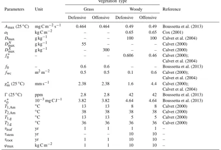
Table 1. Parameterization of vegetation with two strategies.
Vegetation Type
Parameters Unit Grass Woody Reference
Defensive Offensive Defensive Offensive
Amax(25◦C) mg C m−2s−1 0.464 0.464 0.49 0.49 Boussetta et al. (2013)
al kg C m−2 – – 0.65 0.65 Cox (2001)
Dmax g kg−1 – – 100 100 Calvet et al. (2004)
DmaxN g kg−1 55 – – – Calvet (2000)
DmaxX g kg−1 – 300 – – Calvet (2000)
f0∗ – – – 0.606 0.46 Calvet (2000);
Calvet et al. (2004)
f0 – 0.6 0.6 – – Boussetta et al. (2013)
fwc m2m−2 0.5 0.5 0.1 0.6 Calvet (2000);
Calvet et al. (2004) gm∗ (25◦C) mm s−1 2.38 2.38 1.6 4.4 Calvet (2000);
Calvet et al. (2004)
0(25◦C) ppm 2.8 2.8 42 42 Boussetta et al. (2013)
0∗ 10−3mg C J−1 3.82 3.82 4.64 4.64 Boussetta et al. (2013)
T1,Am ◦C 13 13 8 8 Calvet (2000)
T2,Am ◦C 38 38 38 38 Calvet (2000)
T1,g ◦C 13 13 5 5 Calvet (2000)
T2,g ◦C 36 36 36 36 Calvet (2000)
τleaf yr 1 1 1 1 –
τstem yr – – 10 10 –
τroot yr 1 1 10 10 –
ϕmax kg C m−2 1 1 10 10 –
The crown area CA is also used to define a root densityϕ
[kg C m−2], assuming an equal distribution of root biomass over the crown area according to
ϕ=Croot
CA , (10)
which is used to calculate the extractable soil water fraction. Furthermore, it influences the opening of stomata and the sur-face conductivity (more details in Sect. 2.6). A detailed roof profile is not included in the model, similar to the lack of representing a detailed vertical profile of water.
During the photosynthesis simulation, we calculate NPP (see Appendix B). Then based on Eq. (3), the total biomass is updated, after which vegetation structural variables are updated by equations listed in this section. First,Croot and
Cleaf+Cstemcan be calculated for known values ofα(Eq. 5). Second, Cleaf+Cstem can be represented as a function of LAI and CA by combining Eqs. (6) and (7). Then, LAI and CA can be retrieved by the combined equations (Eqs. 6 and 7) and and Eq. (8). Third, CA is compared to CAref. If CA>CAref, LAI will be recalculated by the combined equa-tion while keeping CA=CAref (CA cannot exceed CAref). At last,fc andϕ can be obtained by Eqs. (9) and (10), re-spectively.
2.3 BOSVM model formulation of biomass dynamics and NPP
The total biomass change is controlled by carbon gain from net primary production (NPP) and carbon loss by litter fall (Eq. 3). NPP is equal to gross primary production (GPP) mi-nus dark respiration (Rd). GPP is governed by the photosyn-thetic uptake of carbon, modeled following of the ISBA-A-gs model (Jacobs et al., 1996; Calvet, 2000; Calvet et al., 2004) (see Appendix B for a full description of the photosynthesis model).
LIT is parameterized using an exponential decay of the actual biomass using a predefined residence time due to lit-ter decomposition, which is longer for woody plants than for grass (Table 1).
LIT=Cleaf
τleaf
+Cstem
τstem
+Croot
τroot
, (11)
Table 2. Variables in the main text.
Symbols Unit Contents Symbols Unit Contents
a[v;b] 1 surface albedo of
vegetation (bare ground)
CA m2 crown area
Cveg kg C biomass of vegetation Cleaf kg C biomass of leaf
Croot kg C biomass of root Cstem kg C biomass of stem
D m canopy structure factor E[v;b] kg H2O m−2s−1 evapotranspiration
fc 1 leaf coverage fs 1 relative crown area
fw, fw∗ – extractable water factor
with(out) impact of root density
GPP kg C m−2s−1 gross primary production
G[v;b] W m−2 soil heat flux ga m s−1 aerodynamic
conductance gm m s−1 mesophyll conductance gs,[v;b] m s−1 surface conductance
H[v;b] W m−2 sensible heat flux l E[v;b] W m−2 latent heat flux
LIT kg C m−2s−1 litter production LAI 1 leaf area index
Leak[1;2] kg H2O m−2s−1 water leakage NPP kg C m−2s−1 net primary production
Ps Pa surface pressure P kg H2O m−2s−1 precipitation rate
qa Pa actual vapor pressure qs Pa saturated vapor pressure
Rd kg C m−2s−1 dark respiration RWU 1 relative water use
Rspace 1 relative space of bare soil Rn,[v;b] W m−2 net radiation
Rlwd W m−2 downward longwave radiation Rswd W m−2 downward shortwave radiation
SH kg kg−1 specific humidity at 2 m t s simulation time step
Ta K air temperature at 2 m Ts,[v;b] K surface temperature
T[1;2] K temperature of soil layer 1 and 2
un m s−1 udirection wind speed
vn m s−1 vdirection wind speed W[1;2] kg H2O total water stored in soil layers
α 1 shoot-total biomass ratio θ[1;2] m3H2O m−3 soil moisture
ρa kg m−3 mean air density at constant
pressure
ϕ 1 root density
which is not desirable for our purpose. Another approach as-sumes that NPP allocation is influenced by the availability of resources. For instance, more NPP is allocated to roots under conditions of water and nutrients scarcity, while more NPP is allocated to leaves in light-limited conditions. The method that we used follows LPJ and TRIFFID (Cox, 2001; Sitch et al., 2003), which simulate allocation of NPP by allometric constraints.
Photosynthesis is complex as it is not only determined by environmental elements, but also by the vegetation response to the change of environment. In the A-gs model, the pho-tosynthetic rate is limited by surface temperature, CO2 con-centration, water vapor deficit, incoming solar radiation, and available soil moisture (Calvet, 2000; Calvet et al., 2004). In the BOSVM model we specify an effective extractable soil water fractionfwas a function of soil moisture content and variable root density following
fw=
θ2−θpwp
θcap−θpwp
· ϕ
ϕmax
, (12)
whereθ2[m3m−3] is volumetric soil moisture content in the root layer (second layer, see bottom right panel of Fig. 1);
θpwp, andθcap [m3m−3] are (fixed) soil moisture at wilting point, field capacity, respectively; andϕmaxis the root den-sity leading to the maximum water uptake ability of plants (Table 1). Available water is thus explicitly dependent on the amount of root biomass.
2.4 The surface energy balance and geometric structure of the BOSVM model
In the BOSVM model the energy balance is explicitly simu-lated for two distinct surface fractions (tiles): a bare ground and a vegetation tile (see bottom right panel of Fig. 1). Veg-etation can utilize deep soil water for evapotranspiration, while bare soil has access to a much shallower water reser-voir. For this reason we applied a two-soil layer scheme. The depth of the first and second layer is 0.02 and 0.48 m, respec-tively. Bare soil only can use water from the top layer while vegetation uses the water from the second layer.
Equation (1) can be rewritten for both vegetation and bare soil tiles:
Subscript “v” is used for terms that apply to the vegetation tile, while subscript “b” is used for the bare ground tile.
Net radiationRn,[v;b]is given as
Rn,[v;b]=(1−a[v;b])·Rswd+·Rlwd−·σ·Ts4,[v;b], (14)
whereTs,[v;b][K] is surface temperature;a[v;b][–] is surface
albedo. For bare ground,ab[–] is a constant (0.4), whileav depends on LAI as
av=amin+(amax−amin)·e−k·LAI, (15) whereamin=0.1 [–] andamax=0.4 [–].
Latent heat flux (l E[v;b]) is given by
l E[v;b]=lρa
qs(Ts,[v;b])−qa 1/ga+1/gs,[v;b]
, (16)
where l [J kg H2O−1] is latent heat of vaporization; ρa [kg m−3] is air density at constant pressure; ga [m s−1] is aerodynamic conductance;gs,[v;b][m s−1] is surface conduc-tance;qs [Pa] is surface-saturated specific humidity,qa[Pa] is air specific humidity.
For vegetation, gs,v is equal to the canopy conductance (see Appendix B), while for bare groundgs,bis given by,
gs,b=gs,max·fw∗, (17)
wheregs,max [m s−1] is the maximum surface conductance of bare soil; andfw∗ [–] is extractable water factor of bare ground given by,
fw∗= θ1−θr
θcap−θr
, (18)
whereθ1 [m3m−3] is soil moisture from the top soil layer (first layer),θr=0.01 [m3m−3] is residual soil moisture.
Sensible heat flux is calculated as
H[v;b]=ρacpga Ts,[v;b]−Ta, (19) wherecp[J kg−1K−1] is the specific heat capacity of air; and
Ta[K] is air temperature at 2 m. The soil heat flux is defined as
G[v;b]= −2C1
T1−Ts,[v;b]
z1
, (20)
whereC1 [W m−1K−1] is the thermal conductivity of the soil;T1[K] is the soil temperature of the top soil layer;z1 [0.02 m] is the depth of the first layer. All fluxes are defined as positive downward.
We calculate separate surface temperatures for bare ground and vegetation. However, the soil temperature is iden-tical for the two tiles. Heat flux exchanges between the sur-face and layer 1 are given byG[v;b], while between layer 1 and 2 the heat conductance is parameterized. We assume a zero flux boundary condition below the second layer. The numerical method to update soil temperature is discussed in Appendix C.
2.5 Water balance
As shown in Fig. 1, soil water is recharged by precipitation and can be lost by evapotranspiration and leakage. Consistent with the tiling and two-soil layer structure, the water balance equation can be written as
dW1
dt =z1·CAref
dθ1 dt =
(P−Leak1−Eb·(1−fc))CAref (21) dW2
dt =z2·CAref
dθ2 dt =
(Leak1−Leak2−Ev·fc)CAref, (22) whereW[1;2] [kg H2O] is the total water stored in layer 1
and 2;P [kg H2O m−2s−1] is the precipitation rate; Leak[1;2]
[kg H2O m−2s−1] is water leakage from surface to soil layer 1, and out of the second soil layer to the deep ground, respec-tively; andz2[0.48 m] is the depth of the second soil layer.
Surface runoff is not considered explicitly. Instead, we as-sume that precipitation will infiltrate directly into the second soil layer when soil moisture in the top layer reaches field capacity. Other details are in Appendix D. As the effects of soil type are not taken into account in this study, we keep parameters of soil properties as constants.
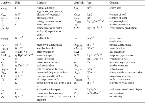
2.6 Soil moisture effects on water use efficiency for the two-soil water stress strategies
In the BOSVM, we include the impact of soil moisture on photosynthesis activity. Observations show that plants can adopt different strategies to cope with drought by control-ling their stomata (Calvet, 2000; Calvet et al., 2004). Dur-ing drought, a class of plants (e.g., soybean, maritime pine; Calvet, 2000; Calvet et al., 2004) close their stomata to de-crease transpiration, but inde-crease mesophyll conductance (gm [m s−1]) to sustain photosynthesis. Another class of plants (e.g., hazel tree, sunflower, sessile oak, Calvet, 2000; Calvet et al., 2004) leave their stomata open for transpiration and decrease the mesophyll conductance. After the soil moisture drops below a threshold, both types start to close stomata and stop carbon assimilation. These strategies affect biomass accumulation significantly and determine different water use efficiencies (WUE) (Eq. 23). More details are described in Calvet (2000) and Calvet et al. (2004). Here we only discuss the relationship between water use efficiency and extractable soil water content.
WUE=GPP
Ev
0 20 40 60 80 100
0.02
0.04
0.06
0.08
0.10
Relative Extractable Water (%)
An /gs
(gC/kgH2O) Def GrassOff Grass Def Woody Off Woody
Fig. 2. Intrinsic WUE as a function of extractable water. Extractable water (fw) is defined as Eq. (12). Solid and dot-dashed lines
represent defensive and offensive strategies, respectively. Thick and thin lines represents grass and woody plants, respectively. vpD = 12 g kg−1, LAI = 1, Rswd=800 W m−2, ca= 380 ppm and
Ts= 25◦C.
In the defensive case, both woody plants and grasses increase WUE when extractable water decreases. Stomata close and gm increases (grass) or maintains (woody) its value. This regime extends until extractable water falls be-low an (observation-based) threshold, from where gm de-creases sharply. The offensive case is more complex. Offen-sive plants insist on maintaining their stomatal opening until very dry conditions are encountered, which is based on the parameterization (Table 1). For woody vegetation,gmthen drops dramatically, which leads to a decrease in photosyn-thesis and consequently a decrease of WUE. However,gmof grass remains relatively constant, which results in a smaller decrease of WUE.
In general, woody plants have a higher water use efficiency than grass. Although WUE of defensive woody vegetation is inversely proportional to soil water content when extractable soil water fractions exceed 10 %, it is still larger than WUE of offensive woody vegetation until extractable water con-tent exceeds 60 %, which is rarely met in arid and semi-arid regimes. Therefore, we assume that the WUE of defensive woody vegetation strategy is always higher than offensive woody vegetation strategy.
2.7 Potential impacts of structural
vegetation parameters on biomass amount
In this study, we explore how vegetation adapts to climate via optimizing its spatial structure (αandD). We assume that the objective of the adaption is that vegetation tries to maximize its total biomass, which is the goal function
α
D
LAI
f
cφ
GPP
R
wuWUE
C
vegpositive negative
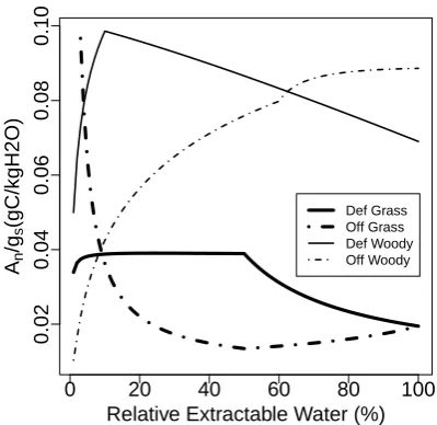
Fig. 3. Impacts ofαandDon vegetation biomass via six variables.
Solid (black) and dashed (red) lines represent positive and nega-tive impact, respecnega-tively.RWUis the relative water use, defined in
Eq. (25).ϕis root density. WUE is water use efficiency as defined in Eq. (23).
Max(Cveg)=f (α, D). (24)
To maximize the total biomass, vegetation structure pa-rameters (α andD) need to be optimized.αandDcannot influenceCveg directly, but determine Cveg via a collection of intermediate variables in the carbon–water–energy cycles. Using the vegetation structure as defined by the parameter-ization of the BOSVM, we illustrate the potential impacts of two structural parameters on total biomass. Biomass amount is updated by carbon gain and carbon loss processes. In the BOSVM, carbon loss is set equal to litter fall (Eq. 3). Since the involved timescalesτleaf,τstemandτroot(Eq. 11) are con-stants, vegetation structure does not affect carbon loss. The amount of carbon gain (NPP) is limited by water and light, where light absorption is directly related to LAI. Concerning the water component, the carbon gain is not only influenced by the degree to which net photosynthesis is governed by available soil water, but also by the ability of vegetation to use water from the neighboring bare ground fraction, which can be represented by the relative water use (RWU).RWUis the ratio of vegetation transpiration over total evapotranspi-ration, defined as
RWU=
Ev·fc
Ev·fc+Eb·(1−fc)
. (25)
From the definition (Eq. 25), we can find that RWU is highly dependent onfc. Notice thatRWUis not equal to rain use efficiency, because water also can be lost by infiltrating deeper soil layers.
WUE depends on extractable soil water content (fw) (Sect. 2.6). From the definition offw(Eq. 12), it is clear that
fwis affected byϕwith given soil moisture.
Figure 3 presents the conceptual relation between struc-tural parameters (αandD), vegetation internal factors (LAI,
Table 3. Constants in the main text.
Symbols Value Contents Symbols Value Contents
a 1.6 diffusivity constants of
H2O and CO2
ab 0.4 albedo of bare ground
amax 0.4 maximum albedo of
vegetation
amin 0.1 minimum albedo of
vegetation
CAref 15 m2 maximum crown area cp 1013 J kg−1K−1 specific heat capacity
of air gs,max 0.2 m s−1 maximum bare ground
conductance
LAIref 6 referred LAI
l 2.45×10⁶J kg−1 latent heat of vaporization SLA 20 m2kg−1 specific leaf area z[1;2] 0.02;0.48 m depth of layer 1 (2) 0.96 surface emissivity θpwp 0.151 soil moisture at wilting
point
θcap 0.346 soil moisture at field
capacity
θr 0.01 residual soil moisture θsat 0.439 saturated soil moisture
σ 5.67×10⁻⁸W m−2K−4 Stefan–Boltzmann constant
(Eq. 5). ϕ declines with an increasing α due to larger CA and lower values ofCroot(Eq. 10). The canopy structure pa-rameterD has a positive impact on LAI and conversely a negative impact onfc, since a high value ofDrepresents a lower crown area. ThereforeDis positively related toϕ for a given value ofα.
A high LAI increases the absorption of light per unit area, which results in a higher GPP. In our two-soil layer scheme (described in Sect. 2.5), bare soil evaporation is only ex-tracted from the top layer. A higherfc reduces water loss from bare soil (Eb(1−fc) in Eq. (25) becomes smaller), which in turn implies thatfchas a positive effect onRWU. A higherfc also implies that the water taken from the bare ground has to be distributed over a larger vegetated area, which imposes a negative effect. This can be expressed by definingRspace, which describes this water distribution frac-tion.
Rspace= 1−fc
fc
(26)
ϕcan have both a positive and a negative impact on WUE, depending on photosynthesis strategies and water content (Sect. 2.6). For offensive grass, a negative relation between
ϕand WUE is present. For other vegetation types, the rela-tion is generally positive. Although WUE decreases when ex-tractable water content exceeds a certain threshold, the mag-nitude of this reduction is relatively low (see Fig. 2).
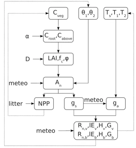
2.8 Simulation process
Figure 4 illustrates the chain of computations followed in the BOSVM model simulation process. The model state variables to be initialized are total biomass, soil moisture and soil temperature in two layers, and a number of veg-etation structure factors before spin up. The initial total biomass is set to 30 kg C to avoid vegetation extinction at
Croot,Cabove
Cveg
α
LAI,fc,φ D
An meteo
NPP gs litter
θ1,θ2 Ts,T1,T2
ga meteo
R
n,v,lEv,Hv,Gv
Rn,b,lEb,Hb,Gb meteo
Fig. 4. Flow diagram of the model. Dashed arrows imply time step updates. For symbols see text.
between high LAI concentrated on a relatively small crown area (CA) or low LAI combined with higher CA. The struc-ture parameterDcontrols this trade-off (Eqs. 7 and 8). Once CA and LAI are known (see method in Sect. 2.2), the vegeta-tion fracvegeta-tion (fc) and root density (ϕ) can be specified (Eqs. 9 and 10).fc is used to define two adjacent tiles (one vege-tated, one bare ground) for which separate energy balances are computed.
The next step is the calculation of the photosynthesis pro-cess, which eventually leads to the specification of the stom-atal conductance (gs) and the biomass gain. Inputs for this photosynthesis calculation are the meteorological forcing, soil moisture conditions and the vegetation structure parame-ters. From soil water content and relative root density we can calculate the mesophyll conductance (gm) and internal CO2 concentration (different approaches used for woody plants and grass, and for defensive or offensive soil moisture strat-egy) as specified in Appendix A. The photosynthesis rate depends on temperature (Appendix B1), internal CO2 con-centration, mesophyll conductance (Appendix B2) and radi-ation (Appendix B3). From the photosynthetic CO2flux (cor-rected for dark respiration) and the gradient of CO2between the ambient atmosphere and the internal concentration, the stomatal conductance can be calculated (Eqs. B10 and B11). This stomatal conductance is upscaled to the canopy scale by applying a vertical integration over the LAI profile (Ap-pendix B4).
The aerodynamic exchange coefficient (ga) is calculated using the Monin–Obukhov similarity theory (Appendix C1). From the meteorological forcing and the aerodynamic and canopy conductance, the energy balance in each tile can be found by solving for the surface temperature (Eqs. 13–20).
The final step in the procedure is the update of the state variables. Vegetation carbon content is updated by the biomass gain from the photosynthesis, and a mortality gov-erned by the litter fall parameterization (Eq. 11). After up-dating theCveg, other structural variables can be updated ac-cording to the method described in Sect. 2.2. The evapotran-spiration rate found in the energy balance algorithm is used to adjust the water balance (Appendix D), while the soil heat flux modifies the soil temperature (Appendix C2). The time step (dt) of the simulation is half an hour for all processes.
2.9 Study area and data sets
The BOSVM model has been set up for a grid configuration covering West Africa, where a large climate gradient exists (see Fig. 5). The model is set up at a 0.5◦ grid and forced
using 3 hourly values of incoming longwave and shortwave radiation, precipitation, air temperature, wind speed and hu-midity for the period 2002 to 2007. The data are generated in the AMMA Land Model Intercomparison Project (Boone et al., 2009), and were used to run and compare a range of land surface models. In this data set, at 10◦E, 15◦N the max-imum annual precipitation is approximately 200 mm yr−1,
−20−5 −10 0 10 20 30
5
15
Annual averaged precipitation (mm/yr)
Longitude
Latitude
1000 2000 3000 4000 ●
● ●
●
−20−5 −10 0 10 20 30
5
15
Incoming shortwave radiation (W/m2)
Longitude
Latitude
180 200 220 240 260
Fig. 5. Annual mean precipitation and incoming shortwave radia-tion distriburadia-tion in West Africa. The four black points are chosen as climate forcings in the second experiment (Sect. 3.2). The rectan-gle marked is the study domain in the third experiment (Sect. 3.3), ranging from 20◦W, 30◦E to 5◦S, 20◦N in West Africa. Data are from the ALMIP forcing data set (Boone et al., 2009).
while it increases to 4000 mm yr−1 near the coast. Short-wave incoming radiation shows an opposite gradient, reduc-ing from 270 W m−2at 20◦N to 170 W m−2near the coast at 5◦N.
Since this study focuses on the effect of vegetation struc-ture on total biomass across a precipitation gradient, the BOSVM model is only applied to a subset of all locations in West Africa. In the second experiment (Sect. 3.2), four grid cells with mean annual precipitation of 200 mm yr−1, 400 mm yr−1, 800 mm yr−1and 1200 mm yr−1(black points in Fig. 5) are chosen as climate forcing to represent the gradi-ent of rainfall. In the third experimgradi-ent (Sect. 3.3), we provide the model simulation for a subregion (the dashed rectangle in Fig. 5).
LAI(m2/m2)
α
D
1 2 3 4 a)
0 0.1 0.2 0.3 0.4 0.5
0.1
0.2
0.5
1.1
2.4
5 Relative CA(m
2
/m2)
α
D
0.2 0.4 0.6 0.8 1.0 b)
0 0.1 0.2 0.3 0.4 0.5
0.1
0.2
0.5
1.1
2.4
5
fc(−)
α
D
0.1 0.2 0.3 0.4 c)
0 0.1 0.2 0.3 0.4 0.5
0.1
0.2
0.5
1.1
2.4
5 Relative ϕ(−)
α
D
0.2 0.4 0.6 0.8 1.0 d)
0 0.1 0.2 0.3 0.4 0.5
0.1
0.2
0.5
1.1
2.4
5
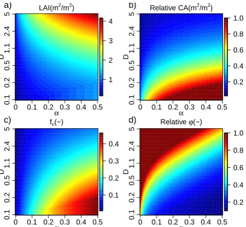
Fig. 6. Patterns of woody vegetation for different combinations ofαandD.αis varied from 0 to 0.5.Dis set from 0.1 to 5. Total biomass
is 30 kg C per pixel of 15 m2. Panel (a): LAI; (b): relative CA; (c):fc; (d): relativeϕ. Relative CA is defined as CA/CAref. Relativeϕis
defined asϕ/ϕmax. Whenϕ > ϕmax, value of relativeϕis set to 1. The scale ofD(y axis) follows an inverse tangent function. Same for
Figs. 7 to 9.
3 Results
3.1 Sensitivity of vegetation structure toαandD
To illustrate the sensitivity of vegetation structure toα and
D, Fig. 6 shows values of LAI,fc, relative CA and relativeϕ for a range ofαandDvalues, assuming a woody vegetation type with constant vegetation biomassCveg=30 kg C for the whole CArefof 15 m2.
LAI increases with bothαandD(Sect. 2.7). Once CA is equal to CAref, LAI has a positive linear relation withα(see bottom left corner of Fig. 6a).
CA and LAI are negatively related for a given amount of leaf biomass (Fig. 6a and b show opposite slopes with certain
α). Both LAI and CA are more sensitive toDwhenα >0.1. Maximum CA appears with highαand lowD. WhenDis extremely low, CAref can be reached by allocating a little amount of leaf biomass. Whenα >0.2, CA is dominated by
Ddue to higher leaf biomass.
fc (Fig. 6c) is dominated by CA. However, it is also af-fected by LAI (Eq. 9), especially when LAI is low. Maximum
fcappears with highαand lowD. Patterns of CA andfcare similar, butfcis more sensitive toα, which has positive re-lations with both CA and LAI (Fig. 3).
ϕ affects the water uptake ability of vegetation (Ap-pendix B). IfCvegis given,ϕdepends onαand CA (Eq. 10). In Fig. 6d, a maximum root density is found with smallαand highD, leading to a large rooting biomass and small crown area.
3.2 Optimal vegetation structure
In this section we simulate how vegetation structure and soil water stress influence biomass, LAI,fc, water use effi-ciency and relative water use (RWU). Ten αand 10 D are chosen to compose an ensemble of 100 vegetation struc-tures. With these ensembles, two-soil water stress strate-gies are applied to four precipitation regimes (200, 400, 800 and 1200 mm yr−1, all ranging within±25 mm yr−1) in West Africa. In each regime approximately five grid points were randomly collected. Here we show simulations for offensive and defensive grass for the 200 mm yr−1climate regime, and woody plant structures for all four climate regimes. The in-trinsic WUE of defensive strategy for woody plants is always higher than that of offensive strategy under same situation (Calvet et al., 2004), which implies that the defensive strat-egy leads to more biomass than the offensive stratstrat-egy with each specific structure. For this reason only the defensive strategy is illustrated for woody plants.
3.2.1 Grass biomass dynamics for 200 mm yr−1
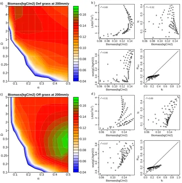
Figure 7a shows the sensitivity of the equilibrium biomass amount for grass as a function ofαandDin the 200 mm yr−1 precipitation regime for the defensive strategy. Figure 7b shows relations ofCveg–LAI,Cveg–fc,Cveg–WUE andfc–
0.04 0.06 0.08 0.10 0.12 0.14 0.16
0.1 0.2 0.3 0.4 0.5
0.1 0.2 0.25 0.3 0.5 1 2 3 4 5
a) Biomass(kgC/m2) Def grass at 200mm/y
α
D 0.06 0.08 0.10 0.12 0.14
1
2
3
4
5
Biomass(kgC/m2)
LAI(
m
2/m 2)
r2
= 0.65 b )
0.06 0.08 0.10 0.12 0.14
0.1
0.2
0.3
0.4
Biomass(kgC/m2)
fc
r2
=−0.32
0.06 0.08 0.10 0.12 0.14
2.8
3.0
3.2
3.4
3.6
Biomass(kgC/m2)
wue(gC/kgH2O)
r2
= 0.66
0.0 0.2 0.4 0.6 0.8 1.0
0.0
0.2
0.4
0.6
0.8
1.0
fc
RW
U
0.04 0.06 0.08 0.10 0.12 0.14 0.16
0.1 0.2 0.3 0.4 0.5
0.1 0.2 0.25 0.3 0.5 1 2 3 4 5
c) Biomass(kgC/m2) Off grass at 200mm/y
α
D 0.06 0.10 0.14
1
2
3
4
5
Biomass(kgC/m2)
LAI(
m
2/m 2)
r2
= 0.31 d )
0.06 0.10 0.14
0.1
0.2
0.3
0.4
Biomass(kgC/m2)
fc
r2
= 0.69
0.06 0.10 0.14
2.6
3.0
3.4
3.8
Biomass(kgC/m2)
wue(gC/kgH2O)
r2
= 0.57
0.0 0.2 0.4 0.6 0.8 1.0
0.0
0.2
0.4
0.6
0.8
1.0
fc
RW
U
Fig. 7.
Sensitivity analysis of equilibrium biomass to vegetation structure: A. Panels
(a)
and
(c)
present
six-year averaged total biomass that changes with different vegetation structures of two strategies.
Pat-terns represent survival structures under the specified regime. Panels
(b)
and
(d)
display several variables
(LAI,
f
cand WUE) as a function of biomass and a comparison between
f
cand
R
WU. Soild lines in Panels
(b)
and
(d)
are one-one line. Panels
(a)
and
(b)
are for defensive grass case under 200 mm yr
−1. Panels
(c)
and
(d)
are for offensive grass case.
58
Fig. 7. Sensitivity analysis of equilibrium biomass to vegetation structure: A. Panels (a) and (c) present 6-year averaged total biomass that changes with different vegetation structures of two strategies. Patterns represent survival structures under the specified regime. Panels (b) and (d) display several variables (LAI,fcand WUE) as a function of biomass and a comparison betweenfcandRWU. Solid lines in panels
(b) and (d) are identity line. Panels (a) and (b) are for the defensive grass case under 200 mm yr−1. Panels (c) and (d) are for the offensive
grass case.
maximumD, which implies a high LAI (2.5 m2m−2) and a very lowfcof 0.06, indicating patches of dense grasses. For defensive grasses , the water use efficiency increases with ex-tractable water (Sect. 2.6 and Fig. 2), implying lowαis more optimal. However, for low values ofα(<0.1), LAI is too low to gain enough carbon to sustain a high root density. A trade-off exists between root density and LAI. Thus the maximum biomass is found for intermediate shoot-total biomass ratio (α=0.15). This also can be seen in Fig. 3. αhas positive and negative impacts on GPP and WUE, respectively, which implies that a trade-off exists. Meanwhile,D has a positive effect on both GPP and WUE, implying that the maximum
Dis optimal. The simulated biomass is more strongly corre-lated with WUE and LAI than withfc(Fig. 7b). We conclude that for dry conditions WUE is more important to biomass thanfc. Moreover, it is interesting to note that the relative
water use (RWU) of the optimized patches (fc=0.06 and
Cveg=0.13 kg C) is higher thanfc. This implies that water is extracted from the surrounding bare soil to supply the tran-spiration from the vegetated fraction of the area.
0.50 0.55 0.60 0.65 0.70 0.75
0.1 0.2 0.3 0.4 0.5
0.1 0.2 0.25 0.3 0.5 1 2 3 4 5
a) Biomass(kgC/m2) Def woody at 200mm/y
α
D 0.3 0.4 0.5 0.6 0.7
0.8
1.2
1.6
2.0
Biomass(kgC/m2)
LAI(
m
2/m 2)
r2
= 0.98 b )
0.3 0.4 0.5 0.6 0.7
0.02
0.03
0.04
0.05
0.06
Biomass(kgC/m2)
fc
r2
= 0.9
0.3 0.4 0.5 0.6 0.7
2.60
2.70
2.80
Biomass(kgC/m2)
wue(gC/kgH2O)
r2
= 0.97
0.0 0.2 0.4 0.6 0.8 1.0
0.0
0.2
0.4
0.6
0.8
1.0
fc
RW
U
0.5 0.6 0.7 0.8 0.9 1.0
0.1 0.2 0.3 0.4 0.5
0.1 0.2 0.25 0.3 0.5 1 2 3 4 5
c) Biomass(kgC/m2) Def woody at 400mm/y
α
D 0.4 0.6 0.8 1.0
0.5
1.0
1.5
2.0
Biomass(kgC/m2)
LAI(
m
2/m 2)
r2
= 0.92 d )
0.4 0.6 0.8 1.0
0.02
0.04
0.06
0.08
Biomass(kgC/m2)
fc
r2
= 0.73
0.4 0.6 0.8 1.0
2.45
2.55
2.65
2.75
Biomass(kgC/m2)
wue(gC/kgH2O)
r2= 0.96
0.0 0.2 0.4 0.6 0.8 1.0
0.0
0.2
0.4
0.6
0.8
1.0
fc
RW
U
Fig. 8.
Sensitivity analysis of equilibrium biomass to vegetation structure: B. As Fig. 7, defensive woody
vegetation case for 200 mm yr
−1(panels
a
and
b) and 400 mm yr
−1(c
and
d).
59
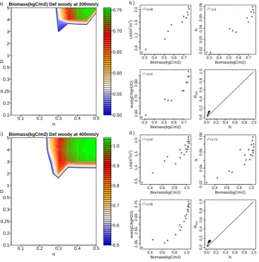
Fig. 8. Sensitivity analysis of equilibrium biomass to vegetation structure: B. As Fig. 7, defensive woody vegetation at 200 mm yr−1(panels
a and b) and 400 mm yr−1(c and d).
WUE is the dominant factor explaining maximum biomass variability (with the highest correlation withCveg). However, some structures also can generate a high WUE with low total biomass. These structures can be found whenα=0.45 and
D≈0.1, where WUE is high but the total amount of water uptake (due to low LAI) is relatively low.
In contrast to the defensive case, thefc of the optimized offensive grasses (fc=0.5) is higher than RWU. It implies that bare soil even “borrows” water from vegetated areas. Compared to the defensive case, less water can be used by the optimized offensive grasses per vegetated area. However, thefcof the optimized offensive grasses is much higher than that of the optimized defensive grasses. Nevertheless, the op-timized defensive grasses have higher biomass per vegetated area (Cveg/fc); the optimized offensive grasses produce more total amount of biomass due to highfc.
3.2.2 Wood biomass dynamics under different precipitation regimes
Figures 8 and 9 show total biomass for woody plants with a defensive drought stress strategy for different climate regimes.
For the 200 mm yr−1precipitation regime, it is clearly il-lustrated that woody biomass has a smaller survival variable space than grasses. Biomass below 0.4 kg C m−2cannot sur-vive due to a minimum GPP needed for maintenance res-piration. The highest biomass is found whenα=0.45 and
D=5. In contrast to defensive grasses, the optimal defen-sive woody structure has a higher biomass due to longer litter timescales and thus slower biomass loss rates.
0.5 1.0 1.5 2.0 2.5 3.0 3.5 4.0
0.1 0.2 0.3 0.4 0.5
0.1 0.2 0.25 0.3 0.5 1 2 3 4 5
a) Biomass(kgC/m2) Def woody at 800mm/y
α
D 1 2 3 4
0.5
1.5
2.5
3.5
Biomass(kgC/m2)
LAI(
m
2/m 2)
r2
= 0.17 b )
1 2 3 4
0.1
0.2
0.3
0.4
0.5
Biomass(kgC/m2)
fc
r2
= 0.91
1 2 3 4
2.4
2.6
2.8
3.0
3.2
Biomass(kgC/m2)
wue(gC/kgH2O)
r2
= 0.35
0.0 0.2 0.4 0.6 0.8 1.0
0.0
0.2
0.4
0.6
0.8
1.0
fc
RW
U
2 4 6 8 10 12
0.1 0.2 0.3 0.4 0.5
0.1 0.2 0.25 0.3 0.5 1 2 3 4 5
c) Biomass(kgC/m2) Def woody at 1200mm/y
α
D 0 2 4 6 8 10 12
0.5
1.5
2.5
3.5
Biomass(kgC/m2)
LAI(
m
2/m 2)
r2
= 0.28 d )
0 2 4 6 8 10 12
0.0
0.1
0.2
0.3
0.4
0.5
Biomass(kgC/m2)
fc
r2
= 0.99
0 2 4 6 8 10 12
2.5
3.0
3.5
4.0
Biomass(kgC/m2)
wue(gC/kgH2O)
r2
= 0.47
0.0 0.2 0.4 0.6 0.8 1.0
0.0
0.2
0.4
0.6
0.8
1.0
fc
RW
U
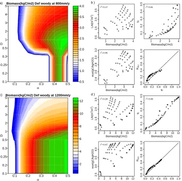
Fig. 9.
Sensitivity analysis of equilibrium biomass to vegetation structure: C. As Fig. 8 for 800 mm yr
−1(panels
a
and
b) and 1200 mm yr
−1(c
and
d).
60
Fig. 9. Sensitivity analysis of equilibrium biomass to vegetation structure: C. As Fig. 8 for 800 mm yr−1(panels a and b) and 1200 mm yr−1
(c and d).
(also see discussion of positive and negative mechanisms in the vegetation–soil water feedback below). As before, it is of interest that theRWUexceeds the vegetation cover. Also, woody vegetation adjusts its environment by using the water from the surrounding bare soil. For both grasses and woody vegetation types, a vertical structure is more beneficial to sur-vive under the dry 200 mm yr−1 regime. Although WUE is the dominant factor explaining total biomass variability, only optimizing WUE is not able to produce high biomass. Wa-ter uptake ability and potential photosynthesis rate are also important.
Figure 8c shows the biomass dependence on vegetation structure for the 400 mm yr−1 precipitation regime. In this wetter regime still many combinations ofDandαlead to a vegetation structure that cannot survive. Figure 8c illustrates that maximum biomass is found at maximum D andα. In the wetter regime, the optimalα is higher and D is lower than that in the 200 mm yr−1regime. Also hereRWU> fc.
Figure 9a shows the results for the 800 mm yr−1 precipita-tion regime. In this wetter regime, some horizontal structures start to survive. With low D (0.1< D <0.3), CA almost reaches CAref, wherefcis strongly regulated by LAI (Eq. 9). Hereαaffects the total biomass drastically. Whenα <0.35, aboveground biomass is too low to gain enough carbon for maintaining root biomass. While ifα >0.45, implying lower
Vertical structure is beneficial to survive, especially in water-limited areas, while it is not able to produce the maximum biomass in wetter regimes. In addition, total biomass is less sensitive to WUE. Instead, leaf coverage becomes the pri-mary factor for optimized biomass.
In the wettest regime (Fig. 9c) most combinations of α
andDcan survive. Plants with lowαcannot survive, as too much carbon is used to maintain the rooting system. Veg-etation with a horizontal structure can survive, and lead to higher biomass.fc andRWUare almost identical (Fig. 9d), implying that water competition between bare and vegetated soil is less important. In this regime, water availability is no constraint and vegetation can survive without using water from the surrounding bare soil. Instead, high leaf coverage can avoid water loss from bare soil evaporation and increase transpiration. Biomass shows a high correlation withfc, im-plying the importance offcto optimize total biomass.
3.3 Dominant factors for different climate regimes
From Sects. 3.1 and 3.2, we found that LAI,fcand WUE in-fluence biomass significantly but their importance is climate dependent. To depict the variability of the response mecha-nisms as a function of the climate regime, we calculate Spear-man’s correlation coefficients between averaged biomass and LAI,fcand WUE under each given climate regime for each vegetation strategy. For each grid cell in the research region (dashed rectangle in Fig. 5) and for each vegetation strategy, we simulate biomass of 100 vegetation structures as defined in Sect. 3.2. Thus we have 100 samples of simulated aver-age biomass, LAI,fcand WUE, which are used to calculate correlation coefficients. Cases where biomass did not survive are not taken into account. Figure 10 presents the variability of the correlation coefficients as a function of mean annual precipitation for four vegetation cases.
From Fig. 10, we can conclude that WUE and LAI are dominant factors in the low precipitation regimes between 200 and 600 mm yr−1, as they generate the highest correla-tion to biomass. LAI generally behaves similarly to WUE. This implies that vegetation requires both a high WUE and a high potential carbon assimilation rate to survive under arid and semi-arid regimes. For low precipitation, vegetation maximizes its biomass by adopting a vertical structure, limit-ingfc. With the increase of precipitation, LAI and WUE are less correlated to biomass, while the correlation ofCvegand
fcincreases (Fig. 10).
3.4 Validation
Our results are validated against observed woody cover data (Hansen et al., 2003; Sankaran et al., 2005). In situ measure-ments of woody cover (Sankaran et al., 2005) are collected from several sites across Africa. The MODIS woody cover product (Hansen et al., 2003) provides a yearly satellite-retrieved tree fraction based on a regression tree algorithm.
200 600 1000 1400
−1.0
−0.5
0.0
0.5
1.0
Defensive Grass
Rainfall(mm/yr)
Correlation coefficient
a)
200 600 1000 1400
−1.0
−0.5
0.0
0.5
1.0
Offensive Grass
Rainfall(mm/yr)
Correlation coefficient
b)
200 600 1000 1400
−1.0
−0.5
0.0
0.5
1.0
Defensive Woody
Rainfall(mm/yr)
Correlation coefficient
c)
Bio−Fc Bio−LAI Bio−WUE
200 600 1000 1400
−1.0
−0.5
0.0
0.5
1.0
Offensive Woody
Rainfall(mm/yr)
Correlation coefficient
d)
Fig. 10. Dominant factor change with precipitation. Correlation co-efficients between averaged biomass and three parameters as a func-tion of mean annual precipitafunc-tion. Panels (a), (b), (c) and (d) repre-sent defensive grass, offensive grass, defensive woody and offensive woody, respectively. Dot-dashed, dashed and solid lines are for cor-relation between biomass andfc, LAI and WUE, respectively.
Here we use a subsample of the MODIS woody cover data developed by Hirota et al. (2011) for validation. We assumed a shoot-total biomass ratio α=0.4, as woody plants with
α=0.4 can more easily survive with horizontal structures (Fig. 9a). Then we chose 10 vegetation canopy structures (Dvaries from 0.2 to 10) and simulated the equilibrium tree cover in the research region (rectangle in Fig. 5).