Open Access
rResearch article
How many repeated measures in repeated measures
designs? Statistical issues for comparative trials
Andrew J Vickers*
Address: Integrative Medicine Service, Biostatistics Service, Memorial Sloan Kettering Cancer Center, Howard 13, 1275 York Avenue NY, NY 10021, USA
Email: Andrew J Vickers* - [email protected] * Corresponding author
Abstract
Background: In many randomized and non-randomized comparative trials, researchers measure a continuous endpoint repeatedly in order to decrease intra-patient variability and thus increase statistical power. There has been little guidance in the literature as to selecting the optimal number of repeated measures.
Methods: The degree to which adding a further measure increases statistical power can be derived from simple formulae. This "marginal benefit" can be used to inform the optimal number of repeat assessments.
Results: Although repeating assessments can have dramatic effects on power, marginal benefit of an additional measure rapidly decreases as the number of measures rises. There is little value in increasing the number of either baseline or post-treatment assessments beyond four, or seven where baseline assessments are taken. An exception is when correlations between measures are low, for instance, episodic conditions such as headache.
Conclusions: The proposed method offers a rational basis for determining the number of repeat measures in repeat measures designs.
Background
Many studies measure a continuous endpoint repeatedly over time. In some cases, this is because researchers wish to judge the time course of a symptom or to evaluate how the effect of a treatment changes over time. For example, in a study of thoracic surgery, patients were evaluated every three months after thoracic surgery to determine the incidence and duration of chronic postoperative pain. The researchers found that the incidence of pain at one year was high and only slightly lower than at three months, showing that post-thoracotomy pain is common and per-sistent[1]. In such studies, the number and timing of repeated measures needs to be decided on a
study-by-study basis depending on the scientific interests of the investigators.
Measures may also be repeated in order obtain a more precise estimate of an endpoint. In simple terms, measure a patient once and they may be having a particularly good or bad day; measure them several times and you are more likely to get a fair picture of how they are doing in general. Repeat assessment reduces intra-patient variability and thus increases study power. This is of particular relevance to comparative studies. For instance, in a randomized trial of soy and placebo for cancer-related hot flashes, patients recorded the number of hot flashes they experienced each
Published: 27 October 2003
BMC Medical Research Methodology 2003, 3:22
Received: 29 August 2003 Accepted: 27 October 2003 This article is available from: http://www.biomedcentral.com/1471-2288/3/22
day during a baseline assessment period and then during treatment. In this case, the researchers were interested in the change between baseline and follow-up in each group so as to determine drug effect. The time course of symp-toms was not at issue. The researchers therefore took a mean of each patient's hot flash score during the baseline period and subtracted the mean of the final four treatment weeks to create a change score. Change scores were com-pared between groups using a t-test [2]. In addition to using means, post-randomization measures may also be summarized by area-under-the-curve [3] or slope scores,[4] which are particularly relevant if treatment effects diverge over time.
There has been little guidance in the methodologic litera-ture as to how researchers should select the number of repeated measures for repeated measures designs. In the few papers that have discussed power and repeat measure-ment (for example, Frison and Pocock[5]), the number of measures is seen as a fixed design characteristic, with sam-ple size derived accordingly. Perhaps as a corollary, rand-omized and other comparative trials involving repeated measures almost invariably lack a statistical rationale for the number of measures taken. Measures are most com-monly taken at particular temporal "landmarks", such as the beginning of each chemotherapy cycle, or each day during treatment. Apparently little consideration is given to how increasing or reducing the number of measures affects power.
Consequently, it is not difficult to find studies that appear to have either too few or too many repeat assessments. In a trial of acupuncture for back pain, for example, pain was measured on a visual analog scale (VAS) once at baseline and once following treatment [6]. The standard deviations were very high: mean post-treatment score was 38 mm with a standard deviation of 28 mm (recalculated using raw data from the authors). Part of this variability in pain scores reflects intra-patient variability that would have been reduced had the VAS been repeated several times. This would surely have been feasible in this population. There are also numerous studies where extremely large number of measures were taken, far beyond the point where additional measures would have improved preci-sion to an important degree. For example, in a trial of a topical treatment for HIV-related peripheral neuropathy, patients were required to record pain four times a day for four weeks at baseline and at follow-up, a total of 224 data points [7]. No rationale was provided for such extensive data collection and there was clearly a cost: 46% of patients dropped-out before the end of the trial. In the hot flashes example given above, symptoms were measured every day for four weeks at baseline and for 12 weeks fol-lowing randomization, a total of 102 data points [2]. The
authors do not explain why such extensive data collection was required to answer the study question.
In this paper I argue that the number of repeat measures should not be seen as a fixed design characteristic, rather it is a design choice that can be informed by statistical con-siderations. I then outline a method for guiding decisions concerning the number of repeat measures and deduce several rules of thumb that can be applied in trial design.
Methods
To determine an optimal number of repeat measures, I use the premise that the ideal number from a statistical viewpoint is infinity, as this would maximally reduce intra-patient variance. However, it would be best in terms of researcher and patient time and effort if only a single assessment was made. Increasing the number of repeat assessments thus has a benefit in statistical terms that is offset by cost. Whereas cost can be estimated only in gen-eral terms by researchers (would patients put up with another questionnaire? how much time would it take for an additional range of motion assessment?) statistical effi-ciency benefits can be quantified. In the following, I describe the formulae for determining the relative benefit of additional repeat assessments for statistical power and deduce some general design principles.
The key question is the degree to which adding a further measure – for example, assessing pain five times rather than four times – increases statistical power. This is known as the "marginal benefit" of repeat measurement. We will start with the situation where data are recorded only after intervention. This is typical in trials of acute sequelae of a predictable event, for example, post-opera-tive pain, chemotherapy nausea or muscle soreness fol-lowing exercise. It can be shown (see Figure 1) that required sample size (n) patients per group is propor-tional to the number of measurements (r) and the mean correlation between measurements ( ).
Marginal change in sample size for r + 1 compared to r assessments is therefore:
This equation does not require that measurements be equally spaced or that correlations between measure-ments be constant.
It is common that trials investigate an endpoint that can be informatively measured before treatment. In trials of
n r
r
∝ +1 ρ( −1)
n n
r r
r+ − r = −
+
1 2
Derivation of statistical formula
Figure 1
Derivation of statistical formula
Take a randomized trial comparing two treatments A and B with ni patients per treatment (i=A, B), in which rpost-randomization assessments are made of a continuous outcome xat times k= 1 … r.The standard model is:
ijk ik
ijk e
x =µ +
Here i= A or B, j= 1 … niandk= 1 … r; µikis the true mean for treatment iat time kandeijk is the error for the jth patient undergoing treatment iat time k.For each patient, a mean of all assessments calculated as:
r k r kΣ=1µ
The difference between groups A and B is:
r Bk Ak r kΣ=1µ −µ
The sample size required for a given power and alpha is proportional to the square of the reciprocal of effect size, d.Effect size is defined as the difference between group means over pooled standard deviation. The variance of the mean ofr assessments is the sum of the variance of each assessment plus twice each pairwise co-variance:
r l k kl r k l r k r k
k ρ σ σ
σ 1 1 1 1 2 2 + = − = = Σ Σ +
∑
Hence effect size is:
l k kl r k l r k r k k Bk Ak r k d σ σ ρ σ µ µ 1 1 1 1 2 1 2 + = − = = = Σ Σ + − Σ =
∑
From the perspective of power, and without loss of generality, the standard deviation of each assessment can be standardized to one, by dividing each xijk by σik. We are not interested in
examining different effect sizes at different times, so we can standardize the difference between groups to one; furthermore, pij can be averaged to give p . Note that there is no requirement for an
assumption that all pij are equal or that kare equally spaced. The number of pairwise correlations
betweenr variables is (r2-r)/2. Hence effect size for r assessments :
) ( 2 r r r r d − + = ρ
Sample size npatients per group is thus:
r r n∝1+ρ( −1)
Marginal change in sample size for r+1 compared to r assessments is therefore:
r r n nr r
+ − = −
+1 2
1
back pain, hypertension or obesity, for example, research-ers want to test whether an intervention reduces patients'
pain scores, blood pressure or weight from a baseline value. Typically the endpoint in such trials is measured
Derivation of statistical formula
Figure 2
Derivation of statistical formula
Sample size for a trial with
p
baseline measures is given by:
−
+
−
−
+
∝
)
1
(
1
)
1
(
1
2p
p
r
r
n
pre mix post
ρ
ρ
ρ
Correlations
pre, post
and
mix
are defined below. As pre-randomization measures are
taken,
k
includes negative values (
-p …
-1, 1
… r).
)
(
2
2 1 1
1
p
p
pre
k lp k l p k
−
Σ
Σ
=
= + − −−
=
ρ
)
(
2
2 1 1
1
r
r
post
klr k l r k
−
Σ
Σ
=
= +−
=
ρ
pr
post
klr l p k
Σ
=Σ
= −=
1 1ρ
For example, given the following correlation matrix:
Pretreatment Posttreatment 1 Posttreatment 2 Posttreatment 3
Pretreatment 1
Posttreatment 1 0.67 1
Posttreatment 2 0.57 0.62 1
Posttreatment 3 0.64 0.47 0.56 1
r
is 3;
p
is 1;
pre
is 1;
post
is the mean of 0.62, 0.47 and 0.56;
mix
is the mean of 0.67,
one or more times at baseline and again following treat-ment. Baseline and post-treatment scores are summarized separately and change analyzed.
Analysis of covariance (ANCOVA) has been repeatedly demonstrated to be the most powerful method of analysis for this type of trial[5,8,9]. The following discussion will thus only include reference to ANCOVA (rather than say, t-test of change between baseline and follow-up). Frison and Pocock[5] have derived a generalized sample size equation that can be used to assess power for ANCOVA where baseline measures are taken before treatment: p is the number of baseline measures; subscripts pre, post and mix refer, respectively, to the mean correlations within baseline measurements, within follow-up measurements and between baseline and follow-up measures (Figure 2).
As is the case for trials without baseline measures, there is no requirement that correlations be equal or that assess-ments be equally spaced.
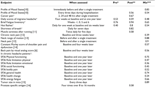
Frison and Pocock report that typical figures for pre, post and mix are 0.7, 0.7, and 0.5. [5] Some figures from my own studies are given in table 1. In general, these data sup-port Frison and Pocock's generalization. Exceptions include episodic conditions, such as headache, in which case correlations are lower, and where the study outcome is measured immediately before and after a single treat-ment session, in which case correlations are higher. The correlations in table 1 can be used to determine the mar-ginal benefit of additional measures for typical trials.
Results
Trials without baseline measures
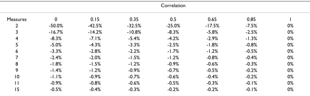
Table 2 shows the marginal relative decreases in sample size given various numbers of assessments and correlations. For example, if correlation between measures is 0.65, increasing the number of measures from two to three decreases sample size requirements by about 6%. As correlation is reciprocally related to intra-patient variability, additional measures are of greatest value when correlation is low. It is also clear that repeating measure-ments more than a few times has little effect on power. For example, for a correlation of 0.65, taking four repeated measures only improves power by 3% compared to three Table 1: Empirical estimates of correlations from a variety of studies
Endpoint When assessed Pre* Post** Mix***
Profile of Mood States[10] Immediately before and after a single treatment 0.83
Profile of Mood States[10] Every three days during hospitalization 0.56 0.54
Cancer pain+ 2, 24 and 48 hrs after single treatment 0.67
Daily scores of migraine headache+ Four weeks at baseline and at one year later 0.53 0.59 0.48
Brief Fatigue Inventory+ Weeks -1, 0, 5 and 6 0.76 0.94 0.65
Hot flashes+ Daily for one week at baseline and six weeks later 0.40 0.8 0.54
Shortness of breath+ Daily for seven days 0.82
Muscle soreness after running [11] Twice daily for five days 0.58
Chronic neck pain [12] Baseline and three weeks later 0.39
Neck range of motion [13] Before and after a single treatment 0.88
Neck pain [13] Before and after a single treatment 0.9
Constant Murley score of shoulder pain and dysfunction [14]
Baseline and four weeks later 0.57
Back pain by visual analog score [6] Baseline and four weeks later 0.56
In chronic headache patients+:
SF36 Physical functioning Baseline and one year later 0.75
SF36 Role limitation physical Baseline and one year later 0.47
SF36 Role limitation emotional Baseline and one year later 0.36
SF36 social functioning Baseline and one year later 0.45
SF36 bodily pain Baseline and one year later 0.52
SF36 general health Baseline and one year later 0.74
SF36 health change Baseline and one year later 0.24
SF36 energy fatigue Baseline and one year later 0.66
Tumor size in mice [15] Every three days 0.89
Prostate specific antigen [16] Four times over 8 to 16 months 0.58
+ unpublished data * Mean correlation between baseline measures **Mean correlation between follow-up measures *** Mean correlation between
baseline and follow-up measures
n r
r
p p
post mix
pre
∝ + − −
+ −
1 1
1 1
2
ρ ρ
ρ
( )
assessments, a negligible value in the context of power calculation.
Trials with baseline measures
Tables 3,4,5 show the effect on sample size of increasing the number of follow-up assessments and baseline assess-ments given different correlations for pre, post and mix. It is assumed for tables 1, 2, 3, 4, 5 that neither the mean of the measures nor the mean correlation between measures depends on the number of measures. This will generally be the case where, for example, a decision needs to be made whether to measure the severity of a chronic condi-tion for one or two weeks at baseline. However, care should be taken with possible exceptions. An example might be if an endpoint was measured twice a day instead of just once. In this case, correlations between
measure-ments 12 hours apart might be higher than those taken 24 hours apart. A second possible exception is acute condi-tions of limited duration: measuring pain after surgery for seven days rather than four days after surgery will not improve precision if few or no patients are in pain after day four.
Table 3 gives the most common situation of moderate cor-relation between baseline and follow-up measures and high correlation within measures. Table 4 shows moder-ate correlation for within and between measures, typical in an episodic condition. Table 5 shows very high correla-tions for studies where assessments are taken close together, or in the case of measures with low intra-patient variability such as laboratory data.
Table 2: Marginal decrease in sample size for increasing the number of measures given various correlations between measures. The table refers to the case where no baseline measures are taken.
Correlation
Measures 0 0.15 0.35 0.5 0.65 0.85 1
2 -50.0% -42.5% -32.5% -25.0% -17.5% -7.5% 0%
3 -16.7% -14.2% -10.8% -8.3% -5.8% -2.5% 0%
4 -8.3% -7.1% -5.4% -4.2% -2.9% -1.3% 0%
5 -5.0% -4.3% -3.3% -2.5% -1.8% -0.8% 0%
6 -3.3% -2.8% -2.2% -1.7% -1.2% -0.5% 0%
7 -2.4% -2.0% -1.5% -1.2% -0.8% -0.4% 0%
8 -1.8% -1.5% -1.2% -0.9% -0.6% -0.3% 0%
9 -1.4% -1.2% -0.9% -0.7% -0.5% -0.2% 0%
10 -1.1% -0.9% -0.7% -0.6% -0.4% -0.2% 0%
11 -0.9% -0.8% -0.6% -0.5% -0.3% -0.1% 0%
15 -0.5% -0.4% -0.3% -0.2% -0.2% -0.1% 0%
Table 3: Sample sizes for various combinations of baseline (p) and follow-up (r) measures. Correlations for pre, post and mix are 0.7, 0.7 and 0.5. Results given relative to a trial with a single baseline and follow-up measure.
Number of baseline measures (p)
No. of follow-up measures (r)
1 2 3 4 5 6 7 8 9 10 12 15
1 100% 94% 92% 90% 89% 89% 88% 88% 88% 88% 87% 87%
2 80% 74% 72% 70% 69% 69% 68% 68% 68% 68% 67% 67%
3 73% 67% 65% 64% 63% 62% 62% 61% 61% 61% 61% 60%
4 70% 64% 62% 60% 59% 59% 58% 58% 58% 58% 57% 57%
5 68% 62% 60% 58% 57% 57% 56% 56% 56% 56% 55% 55%
6 67% 61% 58% 57% 56% 56% 55% 55% 55% 54% 54% 54%
7 66% 60% 57% 56% 55% 55% 54% 54% 54% 53% 53% 53%
8 65% 59% 57% 55% 54% 54% 53% 53% 53% 53% 52% 52%
9 64% 59% 56% 55% 54% 53% 53% 53% 52% 52% 52% 51%
10 64% 58% 56% 54% 53% 53% 52% 52% 52% 52% 51% 51%
12 63% 57% 55% 54% 53% 52% 52% 51% 51% 51% 51% 50%
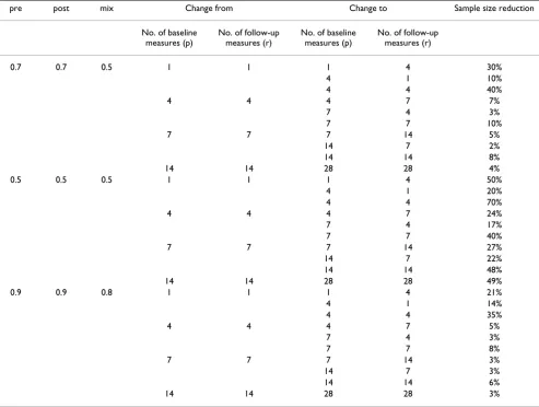
As an example, given the most common case of pre, post and mix at 0.7, 0.7, and 0.5, a trial with four baseline and four follow-up measurements would require 60% of the number of patients of a trial with just one baseline and follow-up; a trial with seven assessments at baseline and follow-up would require 54% as many patients. The same figures are shown in a different format in table 6, which gives the relative decrease in sample size for a number of different combinations of follow-up and or baseline assessments. For example, a trial with seven baseline and follow-up measures would require 10% fewer patients than a trial with four of each type of measure where pre, post and mix are 0.7, 0.7, and 0.5.
Some general patterns emerge:
1. Repeating measures can have dramatic effects on power. Increasing the number of follow-up and / or base-line measures from a single one to three or four can reduce sample sizes by 35 – 70%. However, the increases in power for each additional measure rapidly decreases with increasing number of assessments.
2. Under the assumption that pre and post are similar, it is more valuable to increase the number of follow-up than baseline assessments. This makes intuitive sense: we should be more concerned about the precision of an end-point than a covariate.
3. The marginal value of additional follow-up assessments is higher where baseline measurements are taken. Take the Table 4: Sample sizes for various combinations of baseline (p) and follow-up (r) measures. Correlations for pre, post and mix are 0.5, 0.5 and 0.5. Results given relative to a trial with a single baseline and follow-up measure.
Number of baseline measures (p) No. of follow-up
measures (r)
1 2 3 4 5 6 7 8 9 10 12 15
1 100% 89% 83% 80% 78% 76% 75% 74% 73% 73% 72% 71%
2 67% 56% 50% 47% 44% 43% 42% 41% 40% 39% 38% 38%
3 56% 44% 39% 36% 33% 32% 31% 30% 29% 28% 27% 26%
4 50% 39% 33% 30% 28% 26% 25% 24% 23% 23% 22% 21%
5 47% 36% 30% 27% 24% 23% 22% 21% 20% 19% 18% 18%
6 44% 33% 28% 24% 22% 21% 19% 19% 18% 17% 16% 15%
7 43% 32% 26% 23% 21% 19% 18% 17% 16% 16% 15% 14%
8 42% 31% 25% 22% 19% 18% 17% 16% 15% 14% 13% 13%
9 41% 30% 24% 21% 19% 17% 16% 15% 14% 13% 13% 12%
10 40% 29% 23% 20% 18% 16% 15% 14% 13% 13% 12% 11%
12 39% 28% 22% 19% 17% 15% 14% 13% 12% 12% 11% 10%
15 38% 27% 21% 18% 16% 14% 13% 12% 11% 11% 10% 9%
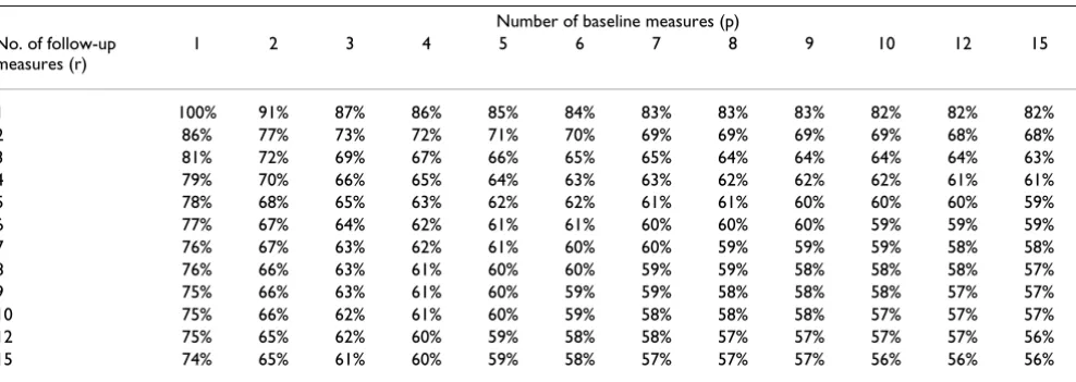
Table 5: Sample sizes for various combinations of baseline (p) and follow-up (r) measures. Correlations for pre, post and mix are 0.9, 0.9 and 0.8. Results given relative to a trial with a single baseline and follow-up measure.
Number of baseline measures (p) No. of follow-up
measures (r)
1 2 3 4 5 6 7 8 9 10 12 15
1 100% 91% 87% 86% 85% 84% 83% 83% 83% 82% 82% 82%
2 86% 77% 73% 72% 71% 70% 69% 69% 69% 69% 68% 68%
3 81% 72% 69% 67% 66% 65% 65% 64% 64% 64% 64% 63%
4 79% 70% 66% 65% 64% 63% 63% 62% 62% 62% 61% 61%
5 78% 68% 65% 63% 62% 62% 61% 61% 60% 60% 60% 59%
6 77% 67% 64% 62% 61% 61% 60% 60% 60% 59% 59% 59%
7 76% 67% 63% 62% 61% 60% 60% 59% 59% 59% 58% 58%
8 76% 66% 63% 61% 60% 60% 59% 59% 58% 58% 58% 57%
9 75% 66% 63% 61% 60% 59% 59% 58% 58% 58% 57% 57%
10 75% 66% 62% 61% 60% 59% 58% 58% 58% 57% 57% 57%
12 75% 65% 62% 60% 59% 58% 58% 57% 57% 57% 57% 56%
case where pre and post are 0.7 and mix is 0.5. For a trial without baseline measures, increasing the number of post-treatment assessments from four to seven decreases sample size by about 4%. The corresponding figures for trials with one or four baseline measures are 6% and 7%. Nonetheless, with the exception of the scenario described in point 4 below, there is little value increasing the number of either baseline or post treatment assessments beyond six or seven.
4. The only situation where it is worthwhile to make more than six or seven assessments is when correlation is mod-erate and similar between all time periods. This is most likely to be the case for episodic conditions such as headache, where scores at any one time will be poorly cor-related with scores at any other time.
Conclusion
Investigators may measure a continuous endpoint repeat-edly because they wish to judge the time course of a symp-tom. In such cases, the number of repeat measures will depend upon the scientific interests of the investigators. Alternatively, investigators may use repeat measurement to increase the precision of an estimate. Though this is a particular concern for randomized or non-randomized comparative studies, it is also pertinent to a variety of other research designs: for example, epidemiologic cohort studies may take a measure such as blood pressure, pros-tate specific antigen or serum micronutrient levels at base-line and then determine whether this predicts development of disease; repeating baselines will improve the precision of such predictions.
Where measures are repeated to improve precision, deci-sions about the number of repeated measures, that is, the number of within-patient observations, mirror those of Table 6: Relative decrease in sample size given various scenarios for increasing the number of baseline (p) or follow-up (r) measures.
pre post mix Change from Change to Sample size reduction
No. of baseline measures (p)
No. of follow-up measures (r)
No. of baseline measures (p)
No. of follow-up measures (r)
0.7 0.7 0.5 1 1 1 4 30%
4 1 10%
4 4 40%
4 4 4 7 7%
7 4 3%
7 7 10%
7 7 7 14 5%
14 7 2%
14 14 8%
14 14 28 28 4%
0.5 0.5 0.5 1 1 1 4 50%
4 1 20%
4 4 70%
4 4 4 7 24%
7 4 17%
7 7 40%
7 7 7 14 27%
14 7 22%
14 14 48%
14 14 28 28 49%
0.9 0.9 0.8 1 1 1 4 21%
4 1 14%
4 4 35%
4 4 4 7 5%
7 4 3%
7 7 8%
7 7 7 14 3%
14 7 3%
14 14 6%
Publish with BioMed Central and every scientist can read your work free of charge "BioMed Central will be the most significant development for disseminating the results of biomedical researc h in our lifetime."
Sir Paul Nurse, Cancer Research UK
Your research papers will be:
available free of charge to the entire biomedical community
peer reviewed and published immediately upon acceptance
cited in PubMed and archived on PubMed Central
yours — you keep the copyright
Submit your manuscript here:
http://www.biomedcentral.com/info/publishing_adv.asp
BioMedcentral standard power calculation, which concerns observations
of separate patients. In both cases, statistical concerns to minimize variance are balanced by logistical concerns to minimize number of assessments. Whilst an extensive lit-erature has developed on various methods for selecting a particular number of patients to study, the number of assessments per patient has received little attention, per-haps because this has tended to be seen as a fixed charac-teristic of any particular trial design. Here I have shown that simple statistical considerations can be used to guide the number of repeated measures in repeated measures designs. Given the most common correlation structure, taking four baselines and seven follow-up measures dra-matically improves power compared to a single baseline and follow-up; where no baseline is taken, four follow-up measures importantly improves power; however, the marginal value of including additional measures rapidly diminishes.
Competing interests
None declared
References
1. Perttunen K, Tasmuth T and Kalso E: Chronic pain after thoracic surgery: a follow-up study. Acta Anaesthesiol Scand 1999,
43:563-567.
2. Van Patten CL, Olivotto IA, Chambers GK, Gelmon KA, Hislop TG, Templeton E, Wattie A and Prior JC: Effect of Soy Phytoestro-gens on Hot Flashes in Postmenopausal Women With Breast Cancer: A Randomized, Controlled Clinical Trial. Jour-nal of Clinical Oncology 2002, 20:1449-1455.
3. Matthews JNS, Altman DG, Campbell MJ and Royston P: Analysis of serial measurements in medical research. BMJ 1990,
300:230-235.
4. Frison LJ and Pocock SJ: Linearly divergent treatment effects in clinical trials with repeated measures: efficient analysis using summary statistics.Stat Med 1997, 16:2855-2872.
5. Frison L and Pocock SJ: Repeated measures in clinical trials: analysis using mean summary statistics and its implications for design.Stat Med 1992, 11:1685-1704.
6. Grant DJ, Bishop-Miller J, Winchester DM, Anderson M and Faulkner S: A randomized comparative trial of acupuncture versus transcutaneous electrical nerve stimulation for chronic back pain in the elderly.Pain 1999, 82:9-13.
7. Paice JA, Ferrans CE, Lashley FR, Shott S, Vizgirda V and Pitrak D:
Topical Capsaicin in the Management of HIV-Associated Peripheral Neuropathy.Journal of Pain and Symptom Management
2000, 19:45-52.
8. Senn S: Repeated measures in clinical trials: analysis using mean summary statistics and its implications for design.Stat Med 1994, 13:197-198.
9. Vickers AJ: The use of percentage change from baseline as an outcome in a controlled trial is statistically inefficient: a sim-ulation study.BMC Med Res Methodol 2001, 1:6.
10. Cassileth BR, Vickers AJ and Magill LA: Music therapy for mood disturbance during hospitalization for autologous stem cell transplantation: a randomized controlled trial.Cancer 2003 in press.
11. Vickers AJ, Fisher P, Smith C, Wyllie SE and Rees R: Homeopathic Arnica 30x is ineffective for muscle soreness after long-dis-tance running: a randomized, double-blind, placebo-control-led trial.Clin J Pain 1998, 14:227-231.
12. Irnich D, Behrens N, Molzen H, Konig A, Gleditsch J, Krauss M, Nata-lis M, Senn E, Beyer A and Schops P: Randomised trial of acupunc-ture compared with conventional massage and "sham" laser acupuncture for treatment of chronic neck pain.BMJ 2001,
322:1574-1578.
13. Irnich D, Behrens N, Gleditsch J, Stor W, Schreiber MA, Schops P, Vickers AJ and Beyer A: Immediate effects of dry needling and acupuncture at distant points in chronic neck pain: results of a randomized, double-blind, sham-controlled crossover trial. Pain 2002, 99:83-89.
14. Kleinhenz J, Streitberger K, Windeler J, Gussbacher A, Mavridis G and Martin E: Randomised clinical trial comparing the effects of acupuncture and a newly designed placebo needle in rotator cuff tendinitis.Pain 1999, 83:235-241.
15. Cheung NK, Modak S, Vickers A and Knuckles B: Orally adminis-tered beta-glucans enhance anti-tumor effects of mono-clonal antibodies.Cancer Immunol Immunother 2002, 51:557-564. 16. Kattan MW, Wheeler TM and Scardino PT: Postoperative
nomo-gram for disease recurrence after radical prostatectomy for prostate cancer.J Clin Oncol 1999, 17:1499-1507.
Pre-publication history
The pre-publication history for this paper can be accessed here: