Analytical Model for Dispersion of Rocket Exhaust –
Source Size Impact Assessment
Bruno K. Bainy1,*, Bardo E. J. Bodmann2, Daniela Buske3, Régis Quadros3
1
Department of Meteorology, Federal University of Pelotas, Pelotas, Brazil 2
Department of Mechanical Engineering, Federal University of Rio Grande do Sul, Porto Alegre, Brazil 3
Department Mathematics and Statistics, Federal University of Pelotas, Pelotas, Brazil
Abstract
This work presents sensitivity tests of a model for calculation of rocket effluent dispersion, with respect to the source size. The model employs the Generalized Integral Laplace Transform Technique (GILTT) to solve, analytically, the advection – diffusion equation. By employing different virtual sources, the point source was changed into volume sources with previously defined crosswind radius (0, 10, 25 and 50 m), and the impact of such modification was assessed in terms of the vertical distribution of atmospheric contaminants and the concentration fields close to the surface. The tests were conducted for cases of stable and unstable planetary boundary layer.Keywords
GILTT, Pollution dispersion, Volume source1. Introduction
The process of launching spacecrafts starts with the ignition, in which the vehicle acquires thrust for a few seconds, followed by the removal of the launching platform, and by leading it to its trajectory. In these first seconds, there is a massive emission of pollutants that are released towards the ground, forming a large, hot and highly toxic cloud. This cloud is called ground cloud and, due to its thermodynamics characteristics, ascend through the troposphere until it reached thermal equilibrium with the environment. The ground cloud is, generally, the object of special interest in what concerns potential risks to human health and safety [1].
Aiming the protection of rockets launching sites, as well as of the inhabitants and sojourners, fauna and flora of the regions adjacent to those sites, it is necessary the use of modelling the dispersion of the emitted contaminants prior to the launching itself, so that the dispersion conditions can be assessed, and the exposure safety criteria can be met. However, because of the high complexity of the processes of formation, ascension, and dispersion of the ground cloud, many considerations and assumptions have been made to simplify the physical problem to solve it. Numerical modelling usually present advantages in terms of the physical representation and increased details regarding the
* Corresponding author:
bkbainy@hotmail.com (Bruno K. Bainy) Published online at http://journal.sapub.org/ajee
Copyright©2018The Author(s).PublishedbyScientific&AcademicPublishing This work is licensed under the Creative Commons Attribution International License (CC BY). http://creativecommons.org/licenses/by/4.0/
atmospheric conditions and chemical processes that occur within it, with the onus of a high computational cost. Analytical (or semi-analytical) models, on the other hand, despite the simplifications they usually embrace (such as wind field), have a good level of accuracy and a low computational cost, and can be used in emergencies, and when a quick output is required.
This work presents the results of sensitivity tests of an analytical model that has been developed for applications at Alcantara Launching Center (ALC), Brazil: the GILTTR (GILTT for Rocket effluent dispersion). The tests were conducted to evaluate the impact the source size (in this case, the ground cloud) exerts on the pollution distribution within the planetary boundary layer (PBL).
2. Methods
The model used is described by the transient two-dimensional advection-diffusion equation, displayed in (1), in which c = c(x,z,t) is the two-dimensional concentration (integrated on the crosswind direction y), u = u(z) is the mean wind speed (aligned to the x axis), Vg is the gravitational settling velocity, and Kx and Kz are, respectively,
the longitudinal and vertical eddy diffusivity coefficients.
(1) The 3D concentration is obtained through (2)
(2)
conditions were set as zero contaminant flux at the top of the PBL, and, at surface, the flux of pollutant was set as proportional to the ground deposition. The source is given by (3), where Q is the rate of contaminant release, Hs is the
source height (the center of the ground cloud), tr is the duration of the pollutant release, η is the Heaviside step function, and δ is the Dirac delta function.
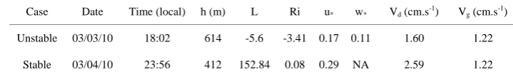
Table 1. Summary of the Cases and Respective Micrometeorological Parameters: PBL Height (h), Monin-Obukhov Length (L), Richardson Number (Ri), Friction Velocity (u*), Convective Scale (w*), Deposition Velocity (Vd), and Gravitational Settling (Vg). NA: Non – Applicable
Case Date Time (local) h (m) L Ri u* w* Vd (cm.s-1) Vg (cm.s-1)
Unstable 03/03/10 18:02 614 -5.6 -3.41 0.17 0.11 1.60 1.22
Stable 03/04/10 23:56 412 152.84 0.08 0.29 NA 2.59 1.22
(3)
The solution is obtained via GILTT, which solves the equation through the following basic steps: expansion of the pollutant concentration in series based on the eigenfunctions of an auxiliary problem, the replacement of this expansion on the advection-diffusion equation, the integration of the equation over the domain of the PBL (taking moments), and the solution of the matrix of the ordinary differential equation system by the Laplace Transform [2]. The mean wind profile was parameterized by the power law [3], and the eddy diffusivity parameters used can be found in [4] for a stable PBL and in [5] for an unstable PBL. More details of the solution, parameterization schemes, and all the modules of this model are given in [6].
The simulations were carried with meteorological data from the Rain Project, collected at the ALC, by means of radiosonde. These data were used as input for the model, for calculation of the micrometeorological and deposition parameters, according to [6]. The summary of the cases is shown on Table 1. The parameters for the source and pollution release are the following: tr = 10 s, Q = 5.2 x 10⁵ g.s-1 of Al2O3, Hs = h*0.5, and Al2O3 density = 3,950 kg.m-3. Simulations were made for four hypothetical source crosswind radiuses (at the release height): 0 m (point source), 10 m, 25 m, and 50 m. This was made by using virtual point sources in various negative distances to produce such previously set radiuses.
3. Results and Discussion
The results of this work are shown on the following. Observed and calculated wind profiles are exhibited in Figure 1. It is noticeable that, in both cases, the model underestimates the windspeed. However, the simulated values express a statistical correlation of 80% for the stable case and 89% for the unstable one. Figure 2 displays the profiles for the eddy diffusivity coefficients, as calculated by the model. The values obtained, as well as their vertical distribution, are according to the expected, meaning that the turbulence is more intense and vertically distributed on the unstable PBL, while the stable PBL presents much lower values, which are maximum on the lower portion of it.
Figure 3 and Figure 4 show the vertical profile of the
crosswind integrated concentration for the stable and unstable cases, respectively. The graphs present the simulated values for x = 1000 m downwind from the source, for different time instants, and for all the considered source radiuses. In both cases, it is perceivable that the differences between the curves (regarding the different radiuses) are initially enhanced and become smaller as time progresses. Undoubtedly, the horizontal advection is the main mechanism of contaminant transport, but the vertical eddies play an important role on the dispersion within an unstable PBL, leading to a better vertical mixture, and, thus, a better dispersion. As consequence, we might see that, on the unstable case (Figure 4), despite the concentrations on the larger initial radiuses reveal smaller concentrations on the middle of the PBL, the respective concentrations are higher on the extremes of the boundary layer (with a particular interest on the ground level proximities). There is no indication that such feature is present on the stable case, in which the vertical transport is much less important.
Figure 1. Observed and simulated wind speed profiles (m.s-1) for the stable (top) and unstable (bottom) cases. Vertical axis displays the non-dimensional height (z/h)
Figure 2. Kz (m2.s-1) versus non-dimensional height for the stable (top) and unstable (bottom) cases
300 s
600 s
1800 s
3600 s
Figure 3. Vertical profile of crosswind integrated concentration versus
non-dimensional height for the stable case
0 2 4 6 8 10 12
0 0.2 0.4 0.6 0.8 1
u observed
u simulated
0 2 4 6 8 10 12
0 0.2 0.4 0.6 0.8 1
u simulated
u observed
0 0.5 1 1.5 2
0 0.2 0.4 0.6 0.8 1
0 20 40 60 80 100
300 s
600 s
1800 s
3600 s
Figure 4. Same as Figure 3, but for the unstable case
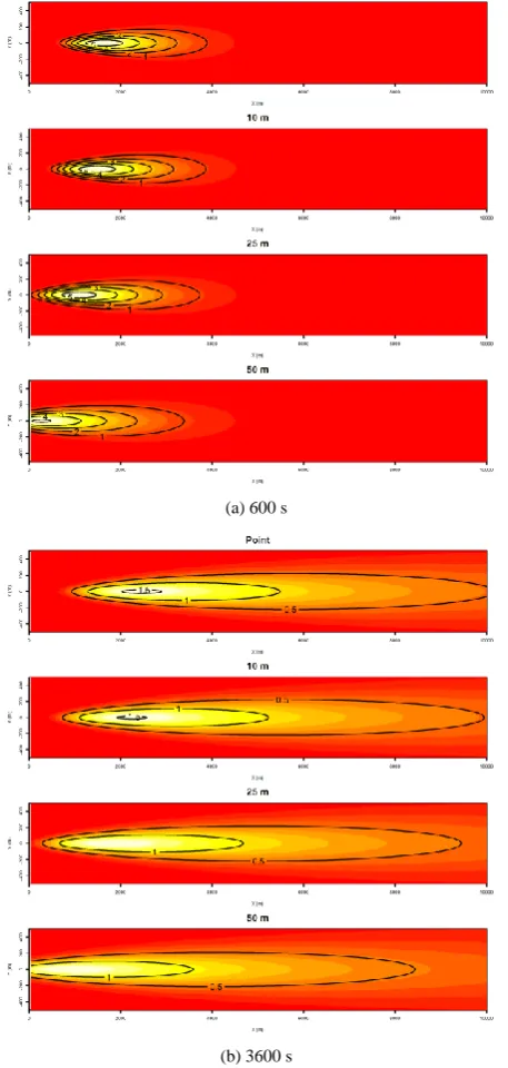
(a) 600 s
(b) 3600 s
Figure 5. Concentrations (mg.m-3) at z = 1 m for the stable case, and the different radiuses and instants
On the unstable PBL, it is perceivable that higher concentrations occur for the simulations with smaller cloud radiuses, and this condition is sustained with time. It is pertinent to point out that the shape and position of the concentration lines, including the centers of maximum concentration, is basically the same for all different radiuses at a given instant of time in the stable case, while there is a sort of lag effect among the unstable cases, regarding the different radiuses, especially for the larger radiuses (not so evident when comparing the point source and the 10 m radius source).
shown), the stable cases features not only much higher concentrations (one order of magnitude higher), which is attributed to the very weak vertical mixture, but also higher concentrations spread horizontally, due to advection effects (reinforcing the discussion of Figure 3, now evident for a much larger area). The opposite happens for the unstable PBL, in which the vertical mixture prevents higher concentrations over a larger horizontal area.
(a) 600 s
(b) 3600 s
Figure 6. Same as figure 5, but for the unstable case
These features may indicate that, concerning human safety in the areas nearby the launching center, the weak vertical mixture of a stable PBL might be the best scenario for rocket launching. Even though for urban applications (car emissions, for instance) a stable layer will keep the pollutants
trapped within the lower levels of the atmosphere, harming human health, we are now considering that the ground cloud ascends within the troposphere, far above ground level. A unstable PBL, oppositely, will contribute to bring the contaminants that ascended in the atmosphere to ground level by means of vertical mixture.
4. Conclusions and Remarks
The results for the sensitivity tests regarding the volume of the emission source were shown, for the cases of a stable and unstable PBL. The model proved itself sensitive in such aspect, as well as presented differences related to the atmospheric stability regime.
There are still improvements to be made in the model, in order to make it more realistic and able to reproduce, with more details, the phenomena inherent to the dispersion processes, especially in cases of rocket launching. However, it must be highlighted that, by using the GILTT, the computational cost of this analytical model is much lower than that of a numerical model, which allows its use in situations when there is need for quick results.
ACKNOWLEDGEMENTS
The authors thank the Brazilian CNPq for funding the research.
REFERENCES
[1] Nyman, R. L., NASA Report: “Evaluation of Taurus II Static Test Firing and Normal Launch Rocket Plume Emissions”, 2009.
[2] Moreira, D. M.; Vilhena, M. T.; Buske, D.; Tirabassi, T., 2009, The state-of-art of the GILTT method to simulate pollutant dispersion in the atmosphere, Atmospheric Research, v. 92, p. 1-17.
[3] Panofsky, H. A.; Dutton, J. A., 1984, Atmospheric Turbulence. John Wiley & Sons. New York, 387 p.
[4] Degrazia, G. A.; Anfossi, D.; Carvalho, J. C.; Mangia, C.; Tirabassi, T.; Velho, H. F. C., 2000, Turbulence parameterisation for PBL dispersion models in all stability conditions. Atmospheric Environment, v. 34, p. 3575–3583. [5] Degrazia G. A., Rizza U, Mangia C, Tirabassi T, 1997,
Validation of a new turbulent parameterization for dispersion models in a convective condition. Boudary Layer Meteorology, v. 85(2), p. 243-254,
doi: 10.1023/A:1000474204748