Numerical Research of the Pollution Surface and Deep-Sea
Evolution in the Sea of Azov Using Satellite Observation Data
T. Ya. Shul’ga*, V. V. Suslin, R. R. Stanichnaya
Marine Hydrophysical Institute, Russian Academy of Sciences, Sevastopol, Russian Federation
*e-mail: [email protected]
Numerical hydrodynamic modeling of the Sea of Azov is done for 2013–2014 on basis of the
Princeton Ocean Model at presetting of real atmospheric impact (the SKIRON model). The hydrodynamic model was applied in numerical studies to analyze the evolution of pollution on the
basis of transport and diffusion equation solution. Level-2 data from MODIS at satellite Aqua with 1
km spatial resolution were used in the work. The following parameters were calculated according to satellite data: the ratio of normalized brightness of the light coming from under the water surface in two 531 and 488 nm spectral channels and light backscattering coefficient by the of the suspension particles at 555 nm wavelength. These data determine the presence of suspended matter (mineral suspended matter from river discharges or rising from the bottom as a result of a strong wind), and suspended matter of biological origin (coccolithophorides bloom). New model algorithms are applied to analyze the consistency of data obtained by remote sensing of the sea surface from space modeling solutions and their combinations. The paper discusses methods of sharing information, assessment of model forecast quality depending on the intervals between satellite data assimilation. It is shown that a serial scheme of data assimilation improves the pollution forecast by the model, even when the satellite images are not stable.
Keywords: Sea of Azov, evolution of passive admixture, remote observations, numerical modeling, comparative analysis of satellite and model data.
DOI: 10.22449/1573-160X-2017-6-36-46
© 2017, T. Ya. Shul’ga*, V. V. Suslin, R. R. Stanichnaya © 2017, Physical Oceanography
Introduction
Ecological problems of the Sea of Azov are given special attention in relation to the continuing significant anthropogenic impact. Pollution scale becomes threat-ening to the ecosystem and results in extremely negative consequences [1]. So, fer-rous and nonferfer-rous metals industries [2–4] are functioning on the Sea of Azov coast. Water transport and dredging, providing the normal functioning of ships in the shallow waters, are among the main sources of the Sea of Azov pollution. The water transport impact on the Sea of Azov ecosystem is quite significant: about 7000 ships pass through navigational canals dug in shallow waters [5].
the comparison of calculations with the operational situation identified by satellite imagery and lead to valid conclusions when making a forecast of pollution spread consequences.
Paper [7] focuses on the numerical study of the Sea of Azov dynamic process impact on the pollution spread. In this paper the main characteristics of wind cur-rents (direction, movement velocity, geometric parameters), direction and the max-imum spread of pollutions are studied on the basis of 3D nonlinear sigma-coordinate Princeton Ocean Model (POM) [8].
In the present work the numerical modeling results and the data of satellite ob-servations of the Sea of Azov water condition over two-year period (2013–2014) are summarized. On the basis of the developed new model algorithms the numeri-cal study of the Sea of Azov spatial-temporal pollution dynamics is carried out. The possibilities of sharing information obtained by methods of the sea surface remote sensing from the space and on the basis of model solutions are discussed. The analysis of modeling and observational data consistency, which allows one to identify negative changes in the marine environment condition, to predict their oc-currence, typical zones and areas covered by anthropogenic impacts is carried out.
The applied mathematical model and its parameters
In the numerical studies a version of 3D nonlinear hydrodynamic model POM
adapted to the Azov basin conditions [9] and also applied for studying the contam-ination evolution under effect of the mentioned disturbances was used. The math-ematical model is based on the equations of a viscous fluid turbulent motion in the hydrostatic approximation [10]. Parameterization of vertical viscosity and turbulent diffusion coefficients is carried out in accordance with semi-empirical differential Mellor-Yamada model with a second-order closure [11]. Horizontal viscosity coef-ficient depending on the horizontal gradients of velocity is calculated using a subgrid viscosity model [12]. The projections of tangential frictional wind stress-es on the free surface are exprstress-essed in terms of wind velocity at a standard meteor-ological height corrected for the sea surface aerodynamic drag coefficient, obtained by formulas expressing empirical dependences on the wind velocity [13]. At the bottom the normal velocity component makes up zero. According to the logarith-mic law, near-bottom tangential stresses are related to the velocity. Using the Grant-Madsen theory [14], the values of the roughness parameter characterizing the hydrodynamic properties of the underlying bottom surface are determined. On the lateral boundaries of the basin, which are assumed to be closed, the adhesion conditions are fulfilled. At the initial time moment fluid motion is absent and free surface is horizontal.
pollution concentration change is carried out as a result of transport and diffusion equation solution. The conditions of absence of admixture fluxes through the side walls, free surface and the basin bottom [8] are added to the dynamic boundary conditions.
Information on the atmospheric pressure and wind fields used in the numerical experiments. Wind and atmospheric pressure fields obtained by the data of
SKIRON regional model over 2013–2014 were used as an atmospheric forcing.
SKIRON atmospheric model was created and developed in the University of Ath-ens by the Atmospheric Modeling and Weather Forecasting Group [16]. It is based on mesoscale numerical atmospheric Eta-model initially developed at the Universi-ty of Belgrade. The main model development was provided by National Centers for Environmental Prediction (NCEP). The results of forecast by SKIRON model applied in this work were obtained by Marine Hydrophysical Institute of RAS as a full participant of Mediterranean Forecasting System Toward Environmental Predictions(MFSTEP) project. This variant of model is a 72 h forecast of meteoro-logical parameters for the Azov – Black Sea and Mediterranean basins. During the first 48 hours the data output is carried out every 2 h, then – every 6 h. The calcula-tion of parameters is performed on the grid with 0.1° step in longitude and latitude. The model provides 16 different parameters including the data on near-water wind.
SKIRON model data were interpolated on the computational grid of the Sea of Azov basin with the mentioned horizontal resolution.
Satellite data preparation
Reconstruction of the Sea of Azov initial hydrooptical initial characteristics by the color scanner data. Methodology of index34 and bbp(555) parameters calcula-tion by the systematized MODIS data. Satellite data for 2013 and 2014 of the
MODIS scanner second level from Aqua satellite [17] with the data rejection ac-cording to certain criteria described in [18] are used in the work. The initial data of instruments were of kilometric spatial resolution. To determine the features in the upper layer of the sea, two parameters were calculated from satellite data. To de-termine the features in the sea upper layer by the satellite data, two parameters were calculated. The first parameter, index34, is a relation of normalized water-leaving radiance LWN(λ) (getting from under the water surface) at λ wave length in two spectral channels: index34 = LWN(531)/LWN(488), where LWN(531) = RRS(531)FO(531), and
LWN(488) = RRS(488)FO(488) (RRS(λ) – the remote-sensing reflectance with central
wavelengths of spectral channels of 531 and 488 nm, respectively; FO(λ) are the solar constants). Physical essence of this parameter consists in the fact that it characteriz-es total absorption of all optically active matters consisting in the seawater upper layer. FO solar constants for the considering spectral channels can be found, for in-stance, in [18].
bbp(555) = [6.76LWN(555) + 0.03(LWN(555))3 + 3.4LWN(555)(I
510)3.8 – 0.84]10–3,
where I510 = LWN(555)/LWN(510). In the course of the study, the data from the Aqua
satellite (with a MODIS scanner onboard) which are freely available on the Internet (http://oceancolor.gsfc.nasa.gov) were used. These data were interpolated on the grid of the mentioned numerical model with 1/59° × 1/84° horizontal resolution in latitude and longitude. Remote data temporal resolution is due to the passage of the satellite (which is daily recorded here at 9 a.m. – 2 p.m. local time) over the Sea of Azov re-gion. The smallest time step between the satellite images is ~24 h.
The most informative images (maximally free from the impact of cloudiness and the presence of omissions) were selected for the analysis from the available satellite data. They are systematized into groups consisting of successive images with the smallest temporal interval between the adjacent ones. The selected periods correspond to good weather conditions over the Sea of Azov water area when the cloudiness is absent. Thus, 6 temporal groups consisting of the most contrast satel-lite images with a discreteness of 1 to 2 days, which were used in the test calcula-tions to estimate the change in the distribution of index34 and bbp(555) parameters under study, are obtained. Three of these groups which are of the greatest interest for the analysis are the data with a daily discreteness, three other – with 2 days in-terval between the images.
For each satellite data temporal group the modeling of distribution of index34 and bbp (555) parameters, which determine the field of suspended matter neutral buoyancy in the near-surface layer of the Sea of Azov, is carried out. Initial bution of these parameters is assimilated in the model by the data of satellite distri-bution in the moment of time coinciding with the first image of group. The model-ing was carried out at a real atmospheric forcmodel-ing (SKIRON) corresponding to the satellite image group of the selected time period. Numerical experiments are car-ried out by two scenarios: without subsequent satellite distribution assimilation of
index34 and bbp(555) parameters and with the assimilation in those moments of time for which satellite data (every 24 or 48 h) are available.
An algorithm for the observational data assimilation
The successive recursive algorithm of data assimilation in the problem of es-timating the passive admixture concentration fields is based on Kalman theory of optimal filtration [20–22]. When solving this problem, in tk moment of time xkm
vector of a priori estimate based on integrating the transport and diffusion equation is constructed. This vector is a short-term model forecast of the investigating pa-rameter from the previous step of assimilation. Its dimension is equal to the number of points of the model space (n = nλnϕ, where nλ = 176 and nϕ = 276 – the number of the grid nodes in longitude and latitude). Satellite observation data comprise yk0
vector of observations. Its dimension (m) varies according to available observa-tional data and does not equal to n in a general case. By the data of observations and the model optimal estimate of xk* concentration is determined using an
algo-rithm of Kalman filter based on forecast – correction system.
We assume that in tk–1 moment of time a forecast of investigated parameter
concentration distribution in the sea surface layer xk–1* is obtained and it is
fore-cast of xkf a priori estimate at tk time moment relying on xk–1*assessment. Then we
obtain y0
k measurements and, correcting the estimate in tk moment, we find the
fi-nal a posteriori assessment of xk* state vector on the basis of the forecast and
meas-urements.
The components of a priori estimate vector xf = (x1f, x2f, …, xnf) are determined
by the found values of the analysis vector x* = (x1*, x2*, …, xn*):
xkf = A(xk-1*) + ξk (k = 1, …, n), (1)
where A is an operator of the model; xk-1* is a vector of analyzed values in tk-1
mo-ment of time (the estimate obtained at (k− 1)th time step) ξ
k is a random vector of
model errors; k is assimilation step. The data of satellite observations constitute the vector y0 = (y0
1, y02, …, y0m):
yk0 = Bkȳ0k + εk (k = 1,…, m), (2)
where Bk is a matrix of model space projections into the observation space of (m × n) dimension; ȳ0
k is m-dimensional vector of observations in tk moment of time; εk is
a random m-dimensional vector of observational errors; The system noise (1) and the one of measurements (2) are Gaussian random processes with zero mathemati-cal expectation. Optimal estimate of xk* concentration is found, according to the
data of the model and measurements, from the condition of the minimum trace of estimation errors covariance matrix on the basis of the Kalman filter algorithm [20–22]:
xk* = xkf + Kk(yk0 – Bkxkf), (3)
Kk = PkfBkT(BkPk
-1*BkT + Rk)–1, (4)
Pkf = Ak
-1Pk-1*Ak-1T + Qk-1. (5)
Here xkf is a concentration forecast over the model; Kk is an unknown weight
ma-trix (Kalman gain) found by the methods of optimal interpolation; Pkf is a of fore-cast error covariance matrix; Rk and Qk-1 are covariance matrices of observational
and model errors, respectively.
The first step of the Kalman filter algorithm consists of the forecast with the computation of preliminary concentration estimate by the formula (1) and the com-putation forecast error covariance matrix (5). Further, by the formula (4) Kk weight matrix is calculated. At the next step of the analysis a desired estimate is deter-mined using the formula (3) based on the data (2) and the analysis error covariance matrix. If the observations are unavailable, we assume that the analysis error covar-iance matrix is equal to the forecast error covarcovar-iance one, and the analysis estimate coincides with the model forecast.
The analysis of numerical experiment results
Comparison of modeling data and satellite images of index34 and bbp(555) pa-rameters distribution in the Sea of Azov. For each temporal group of satellite and modeling data a statistical analysis based on the determination of spatial correlation of index34 and bbp(555) parameters values is carried out. The sets of values of the mentioned parameters are heterogeneous. Satellite data are heterogeneously dis-tributed in space and time. The modeling data obtained on the basis of the transport and diffusion equation integration have a constant discreteness (3 min interval).
The analysis of remote measurement time series. For the analysis of the re-sults, 6 groups of the most informative images obtained in the following periods were selected:
1. April 26 – May 2, 2013 (24–48 h interval between the images). 2. March 21–26, 2014 (24 h interval between the images).
3. August 6–10, 2014 (24 h interval between the images). 4. June 23–29, 2013 (48 h interval between the images). 5. July 17–23, 2014 (48 h interval between the images). 6. November 3–7, 2014 (48 h interval between the images).
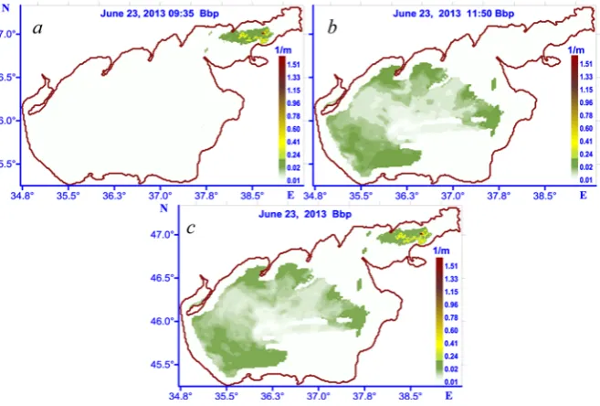
All the satellite data were pre-processed in such a way that if there is a pair of images with 30 min interval from of the same current date, they were concatenated into one image including both of the mentioned ones. For example, the initial im-age of the 4th group was obtained from two consecutive images at 9:35 a. m and
11:50 a. m. on June 23, 2013 (Fig. 1).
Fig. 1. An example of combining the satellite images into one picture. The data of bbp(555) parameter
distribution in the Sea of Azov near-surface layer on June 23, 2013: a – at 9:35 a. m; b – at
11:50 a. m; c – the processed data
pa-rameter. For each period a correlation coefficient (r) of index34 and bbp(555) pa-rameters between the observational data and modeling results in the nodes where there is a data of two considering series was determined. The values of this coeffi-cient, varying within the range from one to zero, determine the data consistency degree. The largest (rmax) and the smallest (rmin) values of cross-correlation
coeffi-cients and time interval, corresponding to the strongest and the weakest correlation in relation to the selected initial parameter in each group, are given in the table.
The analysis of time series reveals that weak correlative dependence primarily occurs in those cases where a large difference in n and m dimensions (at a low-dimensional subspace of observational data) takes place.
Correlation coefficient estimates in the groups of time series satellite data
Group number
Parameter rmax Time interval, h
rmin Time interval, h
1 index34 0.83 120 0.63 25
bbp(555) 0.89 240 0.81 288
2 index34 0.91 72 0.21 96
bbp(555) 0.94 48 0.50 96
3 index34 0.77 72 0.48 24
bbp(555) 0.83 48 0.64 72
4 index34 0.86 96 0.14 120
bbp(555) 0.80 24 0.50 48
5 index34 0.61 24 0.19 264
bbp(555) 0.86 24 0.44 360
6 index34 0.84 48 0.32 96
bbp(555) 0.83 48 0.69 96
The analysis of modeling results and satellite data of admixture evolution in the Sea of Azov depending on the intervals between the satellite data assimilation. During the investigation the modeling of index34 and bbp(555) parameters propaga-tion with the Sea of Azov surface satellite images involvement was carried out. The calculations were performed for the same 6 time groups. As an initial distribution of the studied parameter, its value obtained from the satellite is set in the model. A moment of time in which the assimilation of this initial distribution takes place, corresponds to the date and local time of the existing satellite image.
In Fig. 2 the model and satellite distributions of index34 parameter relating to the first group of images (April 26 – May 2, 2013) are shown. In the left column the satellite images are given, in the right one – the images corresponding to each satellite image of index34 parameter distribution as well as the velocities of surface currents (Fig. 2, c, f, i) according to hydrodynamic model for a close time moment (the difference does not exceed 2 h). Here white areas correspond either to cloudi-ness or to gradient zones which were cut during the data processing. For the model distributions the date and local time are given, in the satellite data a name of the
Wind velocity analysis revealed the fact that approximately two days before the considering time moment (from 24.04.2013, 00:00 a. m.) a northeastern wind with up to 10–12 m/s velocity developed. This wind is the most favorable one for the admixture transport from the Taganrog Bay. The described hydrodynamic sce-nario confirms model distributions of current surface velocity: northeaster wind is accompanied by the currents of the same direction (Fig. 2, c). As can be seen in Fig. 2, d, rather large area in the satellite image is covered with the cloudiness in a day. Modeling data (Fig. 2, e) allow one to assess the character of index34 propa-gation in this area. This figure demonstrates the validity of model forecast at the absence of satellite data. Wind direction changed to the western one, a strip of cur-rents appeared in the central part of the sea. It captured admixture from the shore and transferring it to the center of the basin, to the north and northeast (Fig. 2, f).
At the distributions relating to the time moment of May 2, 2013, 10:00 a.m. (Fig. 2, j) in the region adjacent to the Taganrog Bay and near Berdyansk coast an area of the highest concentration of the considered parameter still takes place. As is obvious (Fig. 2, h), after 6 days from the beginning of assimilation the correspond-ing model distribution poorly reflects the real one.
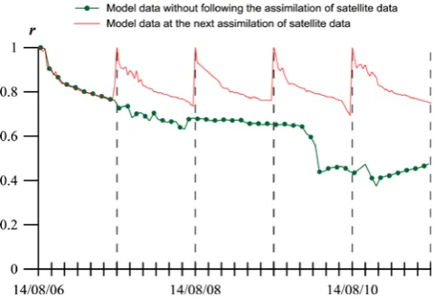
The second series of experiments was carried out to assess the possibilities of assimilation algorithm and to determine its effectiveness with a decrease in the in-terval between the data assimilation. The results of modeling (carried out using a sequential data assimilation procedure) are compared with the ones obtained at a single (initial) assimilation. Assimilation experiments in the selected groups are performed using this algorithm at time moments when informative satellite images exist. Assimilation of index34 and bbp(555) parameters observational data was per-formed applying the Kalman filtering algorithm in which the computation of fore-cast error covariance matrices was carried out by the formula (5). In this experi-ment root-mean-square error of concentration estimate was also determined. It was compared with the same error but obtained during the assimilation of data at the initial time. Thus, the parameter distribution forecast (for example, for 6 days, group 1) was performed in the model by the initial filed (x0m = y00) without
carry-ing out the analysis steps. Root-mean-square error of the forecast was estimated at that. The graphs of the obtained estimations are given in Fig. 3.
The performed analysis of the correlation value between the data of observa-tions and modeling carried out for these two experiments reveals the fact that the assessment of index34 and bbp(555) parameters concentration field with the further assimilation leads to significant decrease of root-mean-square error and to the in-crease of correlation coefficient. It is shown that the successive scheme of observa-tional data assimilation improves the pollution forecast performed according to the model even with unstable satellite images.
Conclusion
A simplified algorithm of data assimilation of admixture concentration observa-tions based on the Kalman filter theory is proposed in the paper. The system of satellite data assimilation consisting of a set of applied programs for determining the passive admixture parameters in the sea surface layer is represented. New algorithms are used in conjunction with the passive admixture transport and diffusion model. The modeling of passive admixture distribution process in the sea is performed on the basis of a set of programs that implement the described algorithm for assimilating observational data. Numerical experiments on assessing the distribution of index34 and bbp(555) parame-ters showed the effectiveness of the algorithms proposed in the work.
The presented numerical algorithms and new program complexes are of practical significance. They can be used to assimilate satellite observations, improve the accura-cy of concentration field determination and have an important property of economy.
Acknowledgements. The work was carried out within the framework the State Order No. 0827-2014-0010 «Complex Interdisciplinary Studies of Oceanographic Processes Determining the Functioning and Evolution of the Black and Azov Sea Ecosystem on the Basis of Modern Methods of Control of the Marine Environment and Gridtehnology» («Fundamental oceanography» code) and the State Order No. 0827-2014-0011 «The research of regularities of marine environment condition changes on the basis of operational observations and the data of marine area condi-tion nowcast, forecast and reanalysis system» («Operative oceanography» code).
REFERENCES
1. Matishov, G.G. and Matishov, D.G., 2013. Current Natural and Social Risks in the Azov-Black
Sea Region. Herald of the Russian Academy of Sciences, [e-journal] 83(6), pp. 490-498.
doi:10.1134/S1019331613090062
2. Klenkin, А.А., Korpakova, I.G., Pavlenko, L.F. and Temerdashev, Z.A., 2007. Ekosistema
Azovskogo Morya: Antropogennoe Zagryaznenie [Ecosystem of the Sea of Azov: Anthropo-genic Pollution]. Krasnodar: Education South Publ., 324 p. (in Russian).
3. Bufetova, M.V., 2015. Zagryaznenie Vod Azovskogo Morya Tyazhelymi Metallami
[Pollu-tion of Sea of Azov with Heavy Metals]. South of Russia: Ecology, Development, [e-journal]
10(3), pp. 112-120 (in Russian). doi:10.18470/1992-1098-2015-3-112-120
4. Matishov, G.G., Berdnikov, S.V., Bespalova, L.A., Ivlieva, O.V., Tsygankova, A.E.,
Khartiev, S.M., Ioshpa, A.R., Arkhipova, O.E., Kropyanko, L.V. [et al.], 2015. Sovremennye
Opasnye Ekzogennye Protsessy v Beregovoy Zone Azovskogo Morya [Modern Dangerous Ex-ogenous Processes in the Coastal Zone of the Azov Sea]. Rostov-on-Don: Southern Federal University, 321 p. (in Russian).
5. Drozdov, V.V., 2010. Osobennosti Mnogoletney Dinamiki Ekosistemy Azovskogo Morya
pod Vliyaniem Klimaticheskikh i Antropogennykh Faktorov [Features of Long-Term Dynam-ics of an Ecosystem of Sea of Azov under the Influence of Climatic and Anthropogenous
Fac-tors]. Uchenye zapiski RSHMU = Proceedings of the Russian State Hydrometeorological
6. Lavrova, O.Yu., Kostianoy, A.G., Lebedev, S.A., Mityagina, M.I. Ginzburg, A.I. and
Shere-met, N.A., 2011. Kompleksniy Sputnikoviy Monitoring Morey Rossii [Complex Satellite
Mon-itoring of the Russian Seas]. Мoscow: SRI RAS, 480 p. (in Russian).
7. Ivanov, V.A., Cherkesov, L.V. and Shulga, T.Ya., 2014. Dynamic Processes and their
In-fluence on the Transformation of the Passive Admixture in the Sea of Azov. Oceanology,
[e-journal] 54(4), pp. 426-434. doi:10.1134/S0001437014030023
8. Blumberg, A.F. and Mellor, G.L., 1987. A Description ofa Three-Dimensional Coastal Ocean
Circulation Model. In: N. Heaps, ed., 1987. Three-Dimensional Coastal Ocean Models.
Washington, D. C.: American Geophysical Union, pp. 1-16. doi:10.1029/CO004
9. Fomin, V.V., 2002. Chislennaya Model' Tsirkulyatsii Vod Azovskogo Morya [Numerical Model
of Water Circulation in the Azov Sea]. In: UHMI, 2002. Scientific Works of UkrNDGMI. Kiev:
Nika-center.Iss. 249, pp. 246-255 (in Russian).
10. Cherkesov, L.V., Ivanov, V.A. and Khartiev, S.M., 1992. Vvedenie v Gidrodinamiku
i Teoriyu Voln [Introduction into Hydrodynamics and Wave Theory]. St. Petersburg: Gidro-meteoizdat, 264 p. (in Russian).
11. Mellor, G.L. and Yamada, T., 1982. Development of a Turbulence Closure Model for
Geo-physical Fluid Problems. Rev. Geophys., [e-journal] 20(4), pp. 851-875.
doi:10.1029/RG020i004p00851
12. Smagorinsky, J, 1963. General Circulation Experiments with Primitive Equations: I. The
Basic Experiment. Mon. Wea. Rev., [e-journal] 91(3), pp. 99-164.
doi:10.1175/1520-0493(1963)091<0099:GCEWTP>2.3.CO;2
13. Wannawong, W., Wongwises, U. and Vongvisessomjai, S., 2011. Mathematical Modeling of
Storm Surge in Three Dimensional Primitive Equations. International Journal of
Mathemati-cal, Computational, PhysiMathemati-cal, Electrical and Computer Engineering, [e-journal] 5(6), pp. 797-806. Available at: http://waset.org/publications/6330/mathematical-modeling-of-storm-surge-in-three-dimensional-primitive-equations [Accessed: 04 July 2017].
14. Grant, W.D. and Madsen, O.S., 1979. Combined Wave and Current Interaction with a Rough
Bottom, J. Geophys. Res., [e-journal] 84(C4), pp. 1797-1808. doi:10.1029/JC084iC04p01797
15. Courant, R., Friedrichs, K.O. and Lewy, H., 1967. On the Partial Difference Equations of
Math-ematical Physics. IBM J. Res. Dev., [e-journal] 11(2), pp. 215-234. doi:10.1147/rd.112.0215
16. Kallos, G., Nickovic, S., Jovic, D., Kakaliagou, O., Papadopoulos, A., Misirlis, N.,
Bou-kas, L., Mimikou, N., Sakellaridis, G., Papageorgiou, J., Anadranistakis, E. and Manousakis, M., 1997. The Regional Weather Forecasting System SKIRON and its Capability for
Fore-casting Dust Uptake and Transport.In: WMO, 1997. Proceedings of the WMO Conference on
Dust Storms, Damascus, 1-6 Nov. Damascus, Syria: WMO, p. 9.
17. NASA Goddard Space Flight Center, Ocean Ecology Laboratory, Ocean Biology
Pro-cessing Group, 2017. Moderate-resolution Imaging Spectroradiometer (MODIS) Aqua
Ocean Color Data; 2014 Reprocessing. Greenbelt, MD, USA: NASA OB.DAAC. doi:10.5067/AQUA/MODIS_OC.2014.0
18. Suslin, V. and Churilova, T., 2016. A Regional Algorithm for Separating Light Absorption by
Chlorophyll-a and Colored Detrital Matter in the Black Sea, Using 480-560 nm Bands from
Ocean Color Scanners. Int. J. Remote Sens., [e-journal] 37(18), pp. 4380-4400.
doi:10.1080/01431161.2016.1211350
19. Suslin, V., Churilova, T., Ivanchik, M., Pryahina, S. and Golovko, N, 2011. A Simple
Ap-proach for Modeling of Downwelling Irradiance in the Black Sea Based on Satellite Data.
Proc. of VI International Conference “Current Problems in Optics of Natural Waters”
(ONW'2011). Saint-Petersburg: Nauka, pp. 199-203.
20. Kalman, R., 1960. A New Approach to Linear Filtering and Prediction Problems. J. Basic
Eng., [e-journal] 82(1), pp. 35-45. doi:10.1115/1.3662552
21. Klimova, E.G., 2003. Numerical Experiments on Meteorological Data Assimilation Using
a Suboptimal Kalman Filter. Russian Meteorology and Hydrology, (10), pp. 40-50.
22. Ghil, M. and Malanotte-Rizzolli, P., 1991. Data Assimilation in Meteorology and
Oceanogra-phy. In: R. Dmowska and B. Saltzman, eds., 1991. Advances in Geophysics. Academic Press.