www.biogeosciences.net/10/7035/2013/ doi:10.5194/bg-10-7035-2013
© Author(s) 2013. CC Attribution 3.0 License.
Biogeosciences
Sea–air CO
2
fluxes in the Indian Ocean between 1990 and 2009
V. V. S. S. Sarma1, A. Lenton2, R. M. Law3, N. Metzl4, P. K. Patra5, S. Doney6, I. D. Lima6, E. Dlugokencky7, M. Ramonet8, and V. Valsala9
1CSIR-National Institute of Oceanography, 176 Lawsons Bay Colony, Visakhapatnam, India
2Centre for Australian Weather and Climate research, CSIRO, Marine and Atmospheric Research, Hobart,
Tasmania, Australia
3Centre for Australian Weather and Climate Research, CSIRO, Marine and Atmospheric Research, Aspendale,
Victoria, Australia
4LOCEAN-IPSL, CNRS Universite Pierre et Marie Curie 4, place Jussieu, 75252 Paris, France 5Reseach Institute for Global Change, JAMSTEC, Yokohama 236 0001, Japan
6Marine Chemistry and Geochemistry, Woods Hole Oceanographic Institution, Woods Hole, MA 02543-1050, USA 7NOAA, Earth System Research Laboratory (ESRL), Global Monitoring Division, Boulder, CO, USA
8Laboratoire des Sciences du Climat et de l’Environnement (LSCE), CEA/CNRS/UVSQ, Gif sur Yvette, France 9Indian Institute of Tropical Meteorology, Dr. Homi Bhabha Road, Pashan, Pune, India
Correspondence to: V. V. S. S. Sarma (sarmav@nio.org)
Received: 16 June 2013 – Published in Biogeosciences Discuss.: 2 July 2013
Revised: 17 September 2013 – Accepted: 26 September – Published: 6 November 2013
Abstract. The Indian Ocean (44◦S–30◦N) plays an im-portant role in the global carbon cycle, yet it remains one of the most poorly sampled ocean regions. Several ap-proaches have been used to estimate net sea–air CO2fluxes
in this region: interpolated observations, ocean biogeochem-ical models, atmospheric and ocean inversions. As part of the RECCAP (REgional Carbon Cycle Assessment and Pro-cesses) project, we combine these different approaches to quantify and assess the magnitude and variability in Indian Ocean sea–air CO2 fluxes between 1990 and 2009. Using
all of the models and inversions, the median annual mean sea–air CO2 uptake of−0.37±0.06 PgC yr−1is consistent
with the −0.24±0.12 PgC yr−1 calculated from observa-tions. The fluxes from the southern Indian Ocean (18–44◦S;
−0.43±0.07 PgC yr−1)are similar in magnitude to the an-nual uptake for the entire Indian Ocean. All models capture the observed pattern of fluxes in the Indian Ocean with the following exceptions: underestimation of upwelling fluxes in the northwestern region (off Oman and Somalia), overesti-mation in the northeastern region (Bay of Bengal) and un-derestimation of the CO2sink in the subtropical convergence
zone. These differences were mainly driven by lack of atmo-spheric CO2data in atmospheric inversions, and poor
simula-tion of monsoonal currents and freshwater discharge in ocean
biogeochemical models. Overall, the models and inversions do capture the phase of the observed seasonality for the en-tire Indian Ocean but overestimate the magnitude. The pre-dicted sea–air CO2fluxes by ocean biogeochemical models
(OBGMs) respond to seasonal variability with strong phase lags with reference to climatological CO2 flux, whereas
the atmospheric inversions predicted an order of magnitude higher seasonal flux than OBGMs. The simulated interannual variability by the OBGMs is weaker than that found by atmo-spheric inversions. Prediction of such weak interannual vari-ability in CO2fluxes by atmospheric inversions was mainly
caused by a lack of atmospheric data in the Indian Ocean. The OBGM models suggest a small strengthening of the sink over the period 1990–2009 of−0.01 PgC decade−1. This is inconsistent with the observations in the southwestern In-dian Ocean that shows the growth rate of oceanicpCO2was
faster than the observed atmospheric CO2growth, a finding
1 Introduction
Since the beginning of the Industrial Revolution, atmospheric carbon dioxide (CO2)concentration has increased with time
due to anthropogenic activities such as fossil fuel combustion and land use changes. These activities led to increased accu-mulation of CO2in the atmosphere from∼4.0 PgC yr−1 in
1970 to 6.8 PgC yr−1in 2000 (Raupach et al., 2007) and up to 8.4 PgC yr−1in 2006 (Boden et al., 2012). Of the total an-thropogenic emissions, about half remain in the atmosphere, leading to warming of the globe in the recent years (IPCC, 2007), and the remaining half is stored in the ocean and on land.
The Indian Ocean is unique compared to the other two ma-jor ocean basins as it is completely closed in the north by the Indian sub-continent and connected to the tropical Pacific via the Indonesian Throughflow (ITF) in the east, and opened to other major oceans at the southern boundary (south of 44◦S; Fig. 1). The northern Indian Ocean (NIO) experiences seasonal reversals in circulation driven by monsoonal forc-ing (Schott and McCreary, 2001), which modulates heat and salinity transport and the biogeochemical cycling of carbon and nitrogen. This zone is one of the most productive regions in the world, accounting for 15–20 % of global ocean pri-mary productivity (e.g., Chavez and Barber, 1987; Behren-field and Falkowski, 1997). Many previous studies on the ocean CO2 system in the Indian Ocean were concentrated
in the northwestern Indian Ocean (Arabian Sea; e.g., George et al., 1994; Kumar et al., 1996; Goyet et al., 1998; Sarma et al., 1996, 1998, 2003) and southwestern Indian Ocean, south of 35◦S (e.g., Metzl et al., 1991; Poisson et al., 1993;
Metzl et al., 1995, 1998; Metzl, 2009). The northeastern re-gion (Bay of Bengal) receives a significant amount of fresh-water and is strongly stratified compared to the northwest-ern Indian Ocean, leading to contrasting behavior in physical processes and biogeochemical cycling (George et al., 1994). Consequently, the northeastern Indian Ocean acts as a mild net sink of atmospheric CO2, whereas the northwestern
In-dian Ocean acts as a net source (Kumar et al., 1996; Sarma, 2003; Takahashi et al., 2009; Valsala and Maksyutov, 2010a; Sarma et al., 2012). The pCO2 in this region shows large
seasonal variations associated with the monsoonal circula-tion, with maxima during summer and winter and minima in the transition periods (Sarma et al., 1998, 2000, 2012; Goyet et al., 1998; Sarma et al., 2003.)
[image:2.595.311.547.64.232.2]In addition to the geographical features, the atmospheric forcing of the Indian Ocean is also unique. The predomi-nant westerly winds can be seen along the Equator in the In-dian Ocean in contrast to the dominant trade winds in other tropical ocean basins. As a result of the existence of west-erly winds in the tropical Indian Ocean, a flat equatorial thermocline is present in the east–west direction that leads to an absence of upwelling in the eastern tropical Indian Ocean with a west-to-east propagation of the annual cycle of
Fig. 1. Sub-regions of the Indian Ocean (30◦N–44◦S, red and blue
combined) used in this paper: northern Indian Ocean (blue), south-ern Indian Ocean (red). The water column circulation pattsouth-ern is also given. East India Coastal Current (EICC), West India Coastal Current (WICC), Somali Current (SC), South Equatorial Counter-current (SECC), East African Coastal Current (EACC), northern East Madagascar Current (NEMC), southern East Madagascar rent (SEMC), South Equatorial Current (SEC), South Java Cur-rent (JC) and Leeuwin CurCur-rent (LC) (Schott and McCreary, 2001). The currents shown in dashed line represent boreal winter, and these currents flow in the opposite direction during boreal sum-mer. Overlain also is the network of atmospheric observations of CO2– Cape Rama, India (CRI); Mount Kenya (MKN); Bukit Koto
Tabang (BKT); Seychelles (SEY); Tromelin Island (TRM); Cape Point (CPT); Amsterdam Island (AMS); Cape Grim Observatory (CGO); Crozet Island (CRZ). The color of the dot indicates how many inversions used data from that location (black: all or almost all inversions; dark grey: around half the inversions; light grey: one or two inversions). We note that the temporal period over which the atmospheric data were collected is not the same for all the stations.
SSTs (sea surface temperatures; Murtugudde and Busalac-chi, 1999; Xie et al., 2002).
The southern tropical and subtropical Indian Ocean are also under the influence of water discharged from the Pa-cific via the Indonesian Through Flow (Valsala and Ikeda, 2007). The region between 15 to 50◦S in the Indian Ocean is a major subduction zone due to positive wind stress curl (Schott et al., 2009). These subducted water masses then travel to the northern Indian Ocean through a shallow merid-ional overturning circulation known as the cross-equatorial cell (Miyama et al., 2003; Schott et al., 2002).
The Indian Ocean remains poorly sampled with respect to CO2spatially, and more importantly temporally. At present
southwest-Fig. 2. The upper figure shows the location of observations of
oceanicpCO2based on 3 million observations collected since 1958
(Takahashi et al., 2009). The lower panel shows the number of months of the year for which observations exist. These data are the basis of the observational data used in this study (reproduced from Takahashi et al., 2009).
ern Indian Ocean, south of 35◦S (e.g., Metzl et al., 1991,
1995, 1998; Poisson et al., 1993; Metzl, 2009).
Nevertheless, several studies do focus on the entire Indian Ocean using interpolation of surface partial pressure of CO2
(pCO2), dissolved inorganic carbon (DIC) and total
alkalin-ity (TA) data collected during the Indian Ocean cruises (e.g., Louanchi et al., 1996; Sabine et al., 2000; Bates et al., 2006). These studies suggest that the region north of 20◦S acts as a strong source of CO2to the atmosphere (0.367 PgC yr−1)
with a sink of atmospheric CO2 between 20 S and 3◦S of
−0.13 PgC yr−1(Bates et al., 2006). This is in contrast with Sabine et al. (2000), who, using underwaypCO2data,
esti-mated the Indian Ocean (north of 35◦S) to be a net sink of atmospheric CO2(−0.15 PgC yr−1)for the year 1995.
Recently Valsala and Makyutov (2013) estimated inter-annual variability in air-sea CO2 fluxes in the NIO using a
simple biogeochemical model coupled to an offline ocean tracer transport model driven by ocean reanalysis data. They found that the maximum seasonal and interannual variability in CO2emissions was located in the coastal Arabian Sea and
southern peninsular India. Valsala et al. (2012) examined the seasonal, interannual and interdecadal variability of atmo-spheric CO2sink in the southern Indian Ocean (SIO). They
reported two distinct CO2uptake regions located between 15
and 35◦S and between 35 and 50◦S. The CO
2 response is
driven by the solubility pump in the northern region, while both the solubility and biological pump contributes equally in the southern region.
The Indian Ocean also experiences strong variability driven by the Indian Ocean Dipole (IOD), and is addition-ally influenced by the El Niño–Southern Oscillation (ENSO) and the Southern Annular Mode (SAM) (Saji et al., 1999; Murthurgude et al., 2002; Thompson and Solomon, 2002). Several physical/hydrological/circulation factors (e.g. vari-ability in atmospheric forcings, open boundaries such as ITF; Fieux et al., 1996; Coatanoan et al., 1999) influence sea–air CO2fluxes and the carbon budgets (Sarma, 2006). The
esti-mated sea–air CO2fluxes at regional and basin scales suggest
strong seasonal and interannual variations (Bates et al., 2006; Goyet et al., 1998; Louanchi et al., 1996; Metzl et al., 1995, 1998, 1999; Sabine et al., 2000; Sarma et al., 1998, 2003; Takahashi et al., 2002, 2009.)
Valsala and Maksyutov (2013) noticed that air-sea CO2
flux anomalies from the coastal Arabian Sea and southern peninsular India are related to the Southern Oscillation (SO) and IOD. When the correlation of CO2flux with the IOD is
stronger, the corresponding correlation with the SO is weaker or opposite. For instance, between 1981 and 1985, about 20 % of interannual variations of CO2emissions in the
Ara-bian Sea were explained by IOD when SO has no significant correlation. On the other hand, between 1990 and 1995, the CO2emissions in the Arabian Sea displayed negative
corre-lation with SO when IOD has no significant recorre-lation. This means that a particular mode is responsible for interannual variation over a group of years. Studies in the southwest-ern Indian Ocean based on long-term CO2observations
de-scribing the spatiotemporalpCO2variations for that region
(Goyet et al., 1991; Metzl et al., 1991, 1995, 1998; Poisson et al., 1993, 1994; Metzl, 2009). In the period 1991–2007 Metzl (2009) calculated an oceanic pCO2 growth rate of
2.11±0.11 µatm yr−1, which is ∼0.4 µatm yr−1faster than in the atmosphere, suggesting that this region acts as a re-ducing sink of atmospheric CO2. They further noted that the
growth rate is similar between 20 S and 42◦S during austral summer (2.2–2.4 µatm yr−1), while it was lower in the north of 40◦S (1.5–1.7 µatm yr−1)than at higher latitudes (> 40◦S) (2.2 µatm yr−1)during austral winter, and such spatial varia-tions were attributed to the SAM.
Gruber et al. (2009) synthesized net air-sea CO2flux
es-timates on the basis of inversions of interior ocean carbon observations, using a suite of ocean generation circulation models and compared these with an oceanic pCO2-based
[image:3.595.50.285.63.341.2]between top-down and bottom-up inversion in the tropical Indian Ocean, potentially due to a lack of atmospheric CO2
data.
Because of the paucity of sampling in this important re-gion, interpolated observations, atmospheric and ocean in-versions, and ocean biogeochemical models have been used to quantify the response of sea–air CO2fluxes over the Indian
Ocean. The objective of this work is to compare the sea–air CO2fluxes and oceanicpCO2from the different approaches
to evaluate and quantify how these simulate CO2 fluxes in
the Indian Ocean on annual mean, seasonal and interannual timescales.
2 Methods
2.1 Study region
Based on the RECCAP regional definitions, we define three primary regions: (i) the entire Indian Ocean (30◦N–44◦S); (ii) the northern Indian Ocean (30◦N–18◦S); and the south-ern Indian Ocean (18–44◦S) (Fig. 1). Additionally, beyond the RECCAP regions we define 3 sub-regions as part of the northern Indian Ocean: the Arabian Sea (0–30◦N, 30– 78◦E); the Bay of Bengal (0–30◦N, 78–100◦E); and the Southern portion of the northern Indian Ocean, as each of these regions have a unique set of key drivers.
2.2 Datasets
In order to describe the regional CO2 fluxes for the Indian
Ocean and its sub-regions, RECCAP Tier 1 global CO2flux
products were used (Canadell et al., 2011), which includes datasets from observations, ocean biogeochemical models, atmospheric and ocean inversions.
2.2.1 Observations
Overall the Indian Ocean remains one of the least sampled basins in the world ocean with respect to CO2measurements
both in terms of space and time (Pfeil et al., 2013). Within the Indian Ocean there are only two zones where data are available: the Arabian Sea, where seasonal data are avail-able, and southwestern Indian Ocean (near Kerguluen Is-lands), where longer-term data are available (Fig. 2). Away from these regions, particularly in the eastern Indian Ocean sparse sampling (2–3 times in a year) makes quantifying and understanding seasonal variability a challenge. In order to fill these gaps, Takahashi et al. (2009) compiled more than 3 million measurements of oceanic pCO2 and these were
averaged onto a global grid (4◦×5◦) with two-dimensional advection–diffusion equations used to interpolate spatially for each month. ThesepCO2data have been interpolated to
[image:4.595.311.544.102.168.2]1◦×1◦grid and combined with the Cross-Calibrated Multi-Platform winds (CCMP; Atlas et al., 2011) to generate a monthly climatology of net sea–air CO2fluxes for RECCAP.
Table 1. The list of ocean biogeochemical models, the periods over
which the data were evaluated and the reference to each model, and the surface area between 30◦N and 44◦S.
Model Name Period Area (km2) Reference
CSIRO∗ 1990–2009 5.06×10⁷ Matear and Lenton (2008) CCSM-BEC∗ 1990–2009 4.28×10⁷ Thomas et al. (2008)
NEMO-Plankton5 1990–2009 5.14×10⁷ Le Quéré et al. (2007) NEMO-PISCES 1990–2009 4.67×10⁷ Aumont and Bopp (2006) CCSM-ETH∗ 1990–2007 4.28×10⁷ Graven et al. (2012) ∗Denotes the models for whichpCO
2values were available.
These fluxes carry several errors associated with sparse cov-erage of data, wind speed measurements and gas transfer co-efficients (see Wanninkhof et al., 2013, and Sweeney et al., 2007, for more discussion). Following Gruber et al. (2009) and Schuster et al. (2013) we estimate the uncertainty on all sea–air flux observations to be ∼50 %. In our subsequent analysis and comparison with different models and inver-sions, we define CO2 flux andpCO2 observations as these
climatologies.
2.2.2 Ocean models
Sea-to-air CO2 flux and oceanicpCO2data were obtained
from five ocean biogeochemical models coupled to ocean general circulation models (Table 1). The models represent physical, chemical and biological processes governing the marine carbon cycle and the exchange of CO2with the
at-mosphere. These models are coarse resolution and do not re-solve mesoscale features. These simulations are driven with meteorological reanalysis products, based on observations, for atmospheric boundary conditions over the period 1990– 2009. All of these models have been integrated from the pre-industrial period to the present day with the same atmo-spheric CO2history. The physical models vary in many
as-pects such as the details of physical forcing, sub-grid scale parameterizations, and experimental configurations that are detailed in the reference for each model in Table 1. In addi-tion, the models incorporate different biogeochemical mod-ules that can substantially influence the simulated fields of surface CO2.
2.2.3 Atmospheric inversions
Atmospheric inversions estimate the surface CO2fluxes that
best fit the spatiotemporal patterns of measured atmospheric CO2 given a defined, time-evolving atmospheric transport
from numerical models. Usually the atmospheric inversions include a priori information about the surface CO2 fluxes,
run globally. Here we focus on those aspects of the inversions pertinent to estimating Indian Ocean fluxes.
While globally the atmospheric inversions typically use measurements from 50 to 100 sites, relatively few are in or near the Indian Ocean region (Fig. 1). The longest records within the region are Seychelles (55◦E, 5◦S) and Amster-dam Island (78◦E, 38◦S), while Cape Point (18◦E, 34◦S) and Cape Grim (145◦E, 40◦S) lie at the edge of the re-gion. Cape Rama (74◦E, 15◦N), Bukit Kototabang (100◦E, 0◦S), Mt Kenya (37◦E, 0◦S) and Tromelin Island (54◦E, 16◦S) have relatively short records within the inversion pe-riod, and many inversions do not include them. Even some of the longer records have suspected data quality issues. Sey-chelles data before 1996 were subject to a variety of sampling methods, with samples likely taken inland between 1994 and 1996 rather than on the coast, making the 1994–1996 mea-surements more susceptible to local effects. Some inversions apply larger data uncertainties to Seychelles data before 1997 for this reason. Amsterdam Island measurements from 2001 to 2005 require correction for calibration issues (Le Quéré et al., 2009), but this correction is not included in most of the data products (e.g., GLOBALVIEW-CO2, 2009) used by the
inversions. Also the GLOBALVIEW-CO2product does not
include Amsterdam Island measurements after 2005, with many inversions consequently relying on extrapolated con-centrations instead. For these reasons, interannual variability from the inversions should be interpreted with caution. To ac-count for these uncertainties in the observational record and potential resulting biases in the calculations of annual mean uptake and variability, we only use values in the period 1997– 2008.
The atmospheric inversions used here estimate carbon fluxes either for pre-defined regions (8 cases) or at the reso-lution of the atmospheric transport model underlying the in-version (3 cases) (Table 2). The number of regions solved for varies across inversions, with 2–10 regions lying fully or par-tially within the Indian Ocean region analyzed here. Where only 2 Indian Ocean regions are solved for, these are close to those defined in Sect. 2.1. For inversions solving at grid-cell resolution, a correlation length scale is used to ensure that the estimated fluxes vary smoothly across larger regions. Most inversions use either the Takahashi et al. (1999) or Takahashi et al. (2009) sea–air CO2fluxes as a prior constraint to the
in-version. These two compilations are similar for the NIO with an annual mean flux of around 0.11–0.12 PgC yr−1, while in the SIO they are a little different (−0.37 or−0.49 PgC yr−1).
Annual mean prior fluxes for the inversions not using these compilations are similar (within 0.1 PgC yr−1 of the
Taka-hashi values).
2.2.4 Ocean inverse methods
Here we use ten ocean inverse model simulations presented by Gruber et al. (2009) and the mean value across these simulations calculated from three periods: 1995, 2000 and
2005. As this technique only solves for an annual mean state, i.e., does not resolve seasonality or interannual variability, these simulations are only used to assess the annual uptake. We have chosen to give all of the models equal weight in order to be consistent with our analysis of ocean models and atmospheric inversions, where no weighting scheme was used. The specific details on methods and models used in these ocean inversions are detailed in Mikaloff Fletcher et al. (2006, 2007) and Gruber et al. (2009).
2.3 Calculation and assessment of sea–air CO2fluxes
Sea–air CO2 fluxes for ocean models and inversions were
calculated as a median and the variability as a median abso-lute deviation (MAD; Gauss, 1816), consistent with Schuster et al. (2013) and Lenton et al. (2013). The MAD is the value where one half of all values are closer to the median than the MAD, and is a useful statistic for excluding outliers in data sets. The calculation of the annual uptake and seasonal variability of sea–air CO2fluxes from atmospheric inversions
and ocean biogeochemical models used data from all of the models and inversions listed in Tables 1 and 2. The sea–air CO2flux into the ocean is defined as negative, consistent with
RECCAP protocols.
3 Result and discussion
In order to examine how well ocean biogeochemical models, ocean and atmospheric inversions are simulating CO2uptake
by the Indian Ocean with reference to observations, compar-isons were made at (i) annual, (ii) seasonal and (iii) interan-nual timescales.
3.1 Annual mean sea–air CO2fluxes for 1990 to 2009
Table 3 and Fig. 3 present the median (across models and inversions) of sea–air CO2flux for the entire Indian Ocean
(44◦S–30◦N), northern Indian Ocean (18◦S–30◦N) and
southern Indian Ocean (44–18◦S). For the atmospheric
in-versions, the annual mean is taken over the available years of each individual inversion, excluding the period before 1997 when some inversions are strongly influenced by poor-quality data at Seychelles. For ocean biogeochemical models, the annual mean was calculated over available years between 1990 and 2009, while in the case of ocean inversions the annual mean flux is calculated from the three periods 1995, 2000 and 2005. The observed pattern of annual mean uptake for the Indian Ocean is shown in Fig. 4.
3.1.1 Entire Indian Ocean (44◦S–30◦N)
The simulated median annual sea–air fluxes varied between
Table 2. The atmospheric inversions and periods over which data were evaluated in this study.
Model Name Period1 Sites used from Fig. 1 Flux res. in Indian2 Reference
LSCE_an_v2.1 1996–2004 5 3.75◦×2.5◦ Piao et al. (2009) LSCE_var_v1.0 1990–2008 6 3.75◦×2.5◦ Chevallier et al. (2010)
C13_CCAM_law 1992–2008 5 10 Rayner et al. (2008)
C13_MATCH_rayner 1992–2008 5 8 Rayner et al. (2008)
CTRACKER_US3 2001–2008 4 4 Peters et al. (2007)
CTRACKER_EU 2001–2008 4 4 Peters et al. (2010)
JENA_s96_v 3.3 1996–2008 3 5◦×3.75◦ Rödenbeck (2005) TRCOM_mean_9008 1990–2008 4 2 Baker et al. (2006)
RIGC_patra 1990–2008 5 4 Patra et al. (2005)
JMA_2010 1990–2008 5 2 Maki et al. (2010)
NICAM_niwa_woaia 1990–2007 6 2 Niwa et al. (2012)4
1Period used for analysis. Inversions may have been run for longer.2Longitude×latitude if inversion solves for each grid cell, otherwise number
of ocean regions in or overlapping the Indian Ocean.3CT2009 release.4Inversion method as this reference, except CONTRAIL aircraft CO2data
[image:6.595.50.547.307.365.2]not used for RECCAP inversion.
Table 3. The annual multi-model median uptake (negative into the ocean) and median absolute deviation (MAD) from ocean biogeochemical
models, atmospheric and ocean inversions, observations and all of the models. All units are PgC yr−1.
Obs OBGC Models Atm Inversions Ocean Inversions All Models (n=26) Surface Area (km2)
30◦N–44◦S −0.24±0.12 −0.36±0.03 −0.36±0.06 −0.37±0.08 −0.37±0.06 4.9×10⁷ 30◦N–18◦S 0.1±0.05 −0.01±0.07 0.13±0.05 0.08±0.01 0.08±0.04 2.44×10⁷ 18◦S–44◦S −0.34±0.17 −0.34±0.06 −0.48±0.03 −0.40±0.02 −0.43±0.07 2.53×10⁷
Fig. 3. Annual median uptake from observations, ocean
biogeo-chemical models, atmospheric inversions and ocean inversions (PgC yr−1). The error bars represent the median absolute deviation (MAD). Negative values represent fluxes into the ocean.
0.1 PgC yr−1compared to observations (−0.24 PgC yr−1), but do agree within the observational uncertainty of
±0.12 Pg yr−1. The observational pattern of CO2 flux in
Fig. 4 shows that the uptake is dominated by the SIO while within the NIO the air-sea flux varies in sign. The near-perfect agreement between the ocean biogeochemical mod-els and the inversions for the entire basin is not maintained
for the NIO/SIO subdivision. The ocean inversions displayed the largest MAD in the annual uptake (0.08 PgC yr−1) fol-lowed by atmospheric inversions (0.06 PgC yr−1), while the smallest MAD was shown by the ocean biogeochemical models (0.03 PgC yr−1; Table 3; Fig. 3). The high MAD in the inversions was caused by sparse atmospheric CO2
mea-surements and differences in the modeled ocean physical cir-culation in the Indian Ocean.
Gruber et al. (2009) synthesized the estimates of the con-temporary net air-sea CO2 flux in the global ocean using
a suite of 10 ocean general circulation models (Mikaloff Fletcher et al., 2006, 2007) and compared them with the TakahashipCO2climatology (Takahashi et al., 2009) for the
period between 1990 and 2000. The difference between the climatology and inversions at the regional level amounted to less than 0.1 PgC yr−1. In addition to this the atmospheric data are available only at four stations in the Indian Ocean (Fig. 1). The reasonable agreement between atmospheric in-versions and oceanpCO2estimates is mainly based on the
prior estimates in the inversion of atmospheric CO2. The
de-viation from these estimates should occur only if these pri-ors turn out to be inconsistent with the atmospheric CO2
data in the context of the inversions. The mismatches be-tween these estimates (inversion versus observations) reflect primarily the relatively small information content of atmo-spheric CO2with regard to regional-scale air-sea CO2fluxes.
[image:6.595.46.290.309.557.2]tem-CSIRO OBS
CCSM-BEC NEMO - Planktom5
CCSM-ETH NEMO - Pisces
[image:7.595.51.286.62.348.2]gC/m2/yr
Fig. 4. Annual mean uptake, in gC m2yr−1, from the five ocean
bio-geochemical models and observations; negative values reflect fluxes into the ocean.
perate Southern Hemisphere, as these regions have an inad-equate number of atmospheric observation stations. As a re-sult, small changes in the selection of the stations (Gurney et al., 2008; Patra et al., 2006) or in the setup of the inversions can lead to large shifts in the inversely estimated fluxes. The ocean regions that seem to be most affected are the tropical Indian Ocean and the temperate South Pacific. Hence, the at-mospheric CO2inversion treats these areas as unconstrained,
and may alter the estimated fluxes substantially in order to match better data constraints elsewhere.
The agreement between observations and all models in the entire basin is not maintained at several zones, namely the Oman/Somali upwelling zone, freshwater discharge zone (Bay of Bengal), the position of the South Equatorial Cur-rent (SEC), uptake in the subtropical convergence zone in the southern subtropical Indian Ocean (Fig. 4). The air-sea CO2 fluxes were poorly simulated by many models in
the northwestern Indian Ocean, where the models underes-timated CO2 fluxes to the atmosphere from the coastal
up-welling zones; in contrast the ocean models overestimated the CO2influx in the freshwater-dominated zone in the Bay
of Bengal. The SEC normally situates at 15–18◦S (Schott and McCreary, 2001) which is the boundary between high surface oceanpCO2and flux to atmosphere and low surface
oceanpCO2and flux into the sea (Sabine et al., 2000). This
transition zone is more easily observed in subsurface features than at the surface, marking the boundary between the low-oxygen, high-nutrient waters of the northern Indian Ocean and the high oxygen, low nutrient values of the subtropical gyre (Wyrtki, 1973). This front marks the northernmost ex-tent of the low surfacepCO2values. This boundary occurred
mostly north of 10◦S by many models. In addition to this, the subtropical convergence zone is the most important CO2
sink zone in the Indian Ocean, and appears underestimated by many models (Fig. 4). The more detailed examination of CO2fluxes in these regions is given below.
3.1.2 Northern Indian Ocean (NIO; 18◦S–30◦N)
Observations suggest that the ocean region north of 10◦S is a net source for atmospheric CO2, i.e., positive sea–air
CO2 flux, with the exception of the Bay of Bengal, which
is a net sink of atmospheric CO2. Encouragingly all
meth-ods, with the exception of the ocean biogeochemical models (OBGMs), simulate a positive sea–air CO2flux over the NIO
region (∼0.1 PgC yr−1; Table 3 and Fig. 3). This net uptake is very consistent with recent water column 14C-dissolved inorganic carbon measurements analyzed over the last 2 decades (0.1±0.03 PgC yr−1; Dutta and Bhusan, 2012). In contrast, OBGMs suggest a small net uptake in this region (−0.01±0.07 PgC yr−1), but do capture areas of strong net positive flux in parts of NIO (Fig. 4). The differences in the NIO may be explained by the location of the transition from net source to sink between the NIO and SIO in OBGMs. Observationally this is located around 18◦S; however all OBGMs suggest that this transition is further northward (mostly north of 10◦S). This means that when the OBGM
uptake estimates are integrated between 30◦N and 18◦S,
we capture areas more characteristic of SIO conditions (i.e., strong net sink) that partially offset the positive sea–air fluxes of CO2 in the NIO, illustrated in Fig. 5. The large source
of CO2 to the atmosphere from the Indian Ocean is driven
by coastal upwelling in the northwestern Indian Ocean, i.e., off Somalia and off the Oman coast, wherepCO2levels as
high as > 600 µatm have been reported during peak south-west (SW) monsoon periods (Kortzinger and Duinker, 1997; Goyet et al., 1998). All models underestimated these fluxes with the exception of NEMO-PLANKTON5, which overesti-mated the flux over the entire NIO. The differences in the re-sponse of the OBGMs in these key regions may be related to challenges of simulating and capturing the observed response by coarse-resolution global models, specifically the mon-soonal circulation and mixing in the Arabian Sea (northwest-ern basin). Here thepCO2levels are highly influenced by the
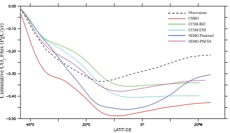
Cumulative CO
2
Flux (PgC/yr)
Observations
CCSM-BEC CSIRO
[image:8.595.51.287.60.197.2]CCSM-ETH NEMO-Plankton5 NEMO-PISCES
Fig. 5. The cumulative, zonally integrated, annual mean CO2
up-take (30◦N–44◦S) from the biogeochemical ocean models and ob-servations (dashed line) (PgC yr−1). Negative values reflect sea–air fluxes into the ocean.
non-monsoon periods (Louanchi et al., 1996; Sarma et al., 2000). Encouragingly, OBGMs in the Arabian Sea do cap-ture the observed net sea–air CO2flux, although the strength
of the source varies among the models.
In contrast several of the ocean prognostic models were capable of simulating the observed CO2sink in the Bay of
Bengal, although again the magnitude varies among mod-els. Both NEMO-PLANKTON 5. and PISCES overestimated and changed the direction of the sea-to-atmosphere flux (Fig. 4). This is recognized as a challenging area to capture the physical and biogeochemical responses related to both the role of the monsoon and the significant amount of dis-charge from the major rivers such as Ganges, Brahmaputra, Godavari, etc., with variable characteristics of an inorganic carbon system. Recently Sarma et al. (2012) observed that whether coastal Bay of Bengal acts as a source or sink may depend on the characteristics of the discharge water received by the coastal zone; in many cases, the current OBGMs either do not incorporate freshwater river inputs at all or treat the lateral river boundary condition as the addition of freshwa-ter only without incorporating explicit wafreshwa-ter chemistry (dis-solved inorganic carbon, alkalinity). The OBGMs underesti-mated the discharge by as much as 50 % (Dia and Trenberth, 2002).
The atmospheric inversions estimate a CO2source to the
atmosphere (0.13±0.05 PgC yr−1)in the NIO which is sim-ilar to that derived from observations. However it is impor-tant to note that the prior ocean flux estimates used by the inversions are also a small source with the majority between 0.11 and 0.12 PgC yr−1(range from 0.05 to 1.14 PgC yr−1).
Since most inversions are using only one set of atmospheric measurements in this region (Seychelles), it is likely that the prior flux has a strong influence on the estimated flux. Dif-ferences in modeled atmospheric transport are also likely to be contribute. Two inversions, C13_CCAM_law and C13_ MATCH_rayner, differ only by the atmospheric transport model used in the inversion and the region map for which
fluxes were solved. However in one inversion, the annual mean flux increased from the prior value and in the other it decreased. These two models show a large difference in the CO2response at Seychelles due to the prior land flux, and
this is compensated in the inversion by altering the ocean flux local to Seychelles. This emphasizes the challenge for atmo-spheric inversions in this region, where both the ocean region itself has limited atmospheric observations and the surround-ing land regions are also very poorly sampled, if at all.
Gruber et al. (2009) compared the “top-down” estimates of the air-sea fluxes based on the interannual inversions of atmospheric CO2with the “bottom-up” estimates based on
the oceanic inversion or the surface oceanpCO2data. They
found excellent agreements in many regions except the trop-ical Indian Ocean (18◦S–18◦N) and temperate Southern Hemisphere. The mismatches between these two estimates reflect information on atmospheric CO2 with regard to
air-sea CO2fluxes (Jacobson et al., 2007).
3.1.3 Southern Indian Ocean (SIO; 44–18◦S)
This region comprises two key oceanographic regimes: the oligotrophic waters in the northern part and Southern Ocean waters in the south. The Subtropical Front (STF) separates these two regimes nominally at 40◦S in this region. In-tegrated over these regions, the median of all approaches (−0.43±0.07 PgC yr−1) suggests a strong sink of atmo-spheric CO2that agrees within observational uncertainty in
this region (−0.34±0.17 PgC yr−1). The median of OBGMs (−0.34±0.06 PgC yr−1) agrees particularly well with the observed CO2 flux. Conversely the atmospheric inversions
estimate a larger uptake (−0.48±0.03 PgC yr−1), while the
oceanic inversions estimates (−0.40±0.02 PgC yr−1)lie
be-tween these values. It is worth noting that even the larger up-take estimated by the atmospheric and ocean inversions lies within the uncertainty of the observed flux. The SIO fluxes are similar in magnitude to the annual uptake for the entire Indian Ocean, indicating the majority of the net uptake oc-curs in the SIO, consistent with other studies (Sabine et al., 2000; Bates et al., 2006; Metzl, 2007; Takahashi et al., 2009). OBGMs (Fig. 4) clearly show the response of the two oceanographic regimes: in the oligotrophic waters a net an-nual sink of CO2 is evident, while south of the STF a
sig-nificantly stronger net sink is seen, consistent with observa-tions (Metzl, 2009, and references therein). However, the flux magnitudes were not well represented with reference to ob-servations. For instance, in the 30–40◦S latitudinal belt, the
oceanic uptake of CO2was underestimated compared to the
the interior of the ocean. Overestimation of the CO2uptake
by the models in these zones suggests that vertical mixing was not constrained properly in the models, leading to ex-cess deep mixing, which resulted in an increase in surface waterpCO2and a decrease in the flux to the ocean.
In the case of atmospheric inversions, there is more vari-ation in prior flux for the SIO than for the NIO. Most in-versions used a prior of either−0.37 or−0.49 PgC yr−1, re-flecting changes in Takahashi et al. (2009) fluxes compared with earlier compilations. The ensemble of inversions did not reconcile this difference, with estimated SIO fluxes span-ning a larger range than the range of prior fluxes. As for the NIO, the SIO was poorly constrained by atmospheric mea-surements. The key site for the SIO region is Amsterdam Is-land, but this was not used in all inversions and, as noted in Sect. 2.2.3, there are some issues about data availability and calibration from 2000 onwards. It is likely that atmo-spheric transport differences also contributed to the variabil-ity in uptake estimates for this region. Gruber et al. (2009) noted that the temperate region of the Indian Ocean in the Southern Hemisphere (18–44◦S) had excellent agreement between ocean inversions and atmospheric inversions, more so with TRANSCOM T3L3 interannually resolved inver-sions (Baker et al., 2006) than with TRANSCOM T3L1, which only solved for mean fluxes (Gurney et al., 2003). Though the actual reasons are unknown for why interannual inversions agreed better with the bottom-up estimates than those inversions solving only for mean fluxes or mean sea-sonality, they hypothesized that selection of the time period of data used and selection of observation stations were po-tential causes (Patra et al., 2006; Gurney et al., 2008).
3.2 Seasonal variations inpCO2and sea–air CO2fluxes
In order to examine how well various modeling approaches simulate seasonal variations in air-sea CO2 fluxes with
re-spect to observations in the Indian Ocean, the simulated
pCO2by different models was compared with observations.
This provides insights into the ability of ocean biogeochemi-cal models to represent the complex interplay of physibiogeochemi-cal and biological processes that drive sea–air CO2 exchange. The
ability of a model to reproduce the seasonal cycle also pro-vides some reassurance that the ocean models are correctly projecting climate sensitivity of the processes that could in-fluence long-term projections of the ocean CO2uptake.
3.2.1 Indian Ocean 44◦S–30◦N
In June to September, the changes in air-sea CO2 fluxes in
the Indian Ocean result from the combined effects of in-creased mixing driven by southwest monsoon, resulting in increased biological uptake of CO2in the NIO, while deeper
mixing and low production, offset to some degree by sur-face cooling, result in a increasedpCO2 levels in the SIO
(Louanchi et al., 1996; Sarma et al., 2000; Takahashi et al.,
30N-44S
18S-44S 30N-18S
Ocean Biogeochemical Models Atmospheric Inversions Observations
Ocean Biogeochemical Models Atmospheric Inversions Observations
Ocean Biogeochemical Models Atmospheric Inversions Observations
Fig. 6. Seasonal cycle anomaly of the Indian Ocean CO2 flux
(PgC yr−1)from observations, ocean biogeochemical models, and atmospheric inversions for the entire Indian Ocean (30◦N–44◦S upper), northern Indian Ocean (30◦N–18◦S middle) and the south-ern Indian Ocean (18–44◦S; lower).
2009). Figure 6 shows the median and MAD air-sea flux sea-sonal cycle anomaly across ocean models and atmospheric inversions compared to the seasonality derived from obser-vations. In general the ocean models and atmospheric inver-sions capture the phasing of the observed seasonality for the entire Indian Ocean (Fig. 6) but overestimate the magnitude. The variation across ocean models is smaller than the vari-ation across inversions. This varivari-ation will be explored in Sect. 3.2.2 and Sect. 3.2.3 when the seasonality of fluxes for the NIO and SIO are presented. The seasonality for the en-tire Indian Ocean was dominated by the seasonality in the SIO. The seasonal variationspCO2 for individual OGBMs
were drawn for the entire Indian Ocean in Fig. 7. Ocean bio-geochemical models captured the observed seasonal cycle for the Indian Ocean; however all individual models over-estimate the magnitude of thepCO2seasonality in all
sea-sons, consistent with the larger-than-observed median annual mean uptake.
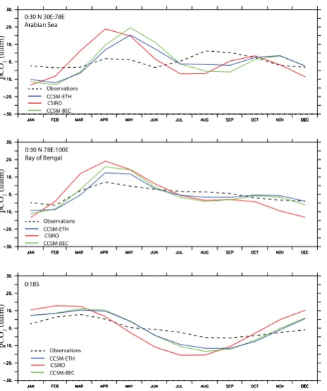
3.2.2 North Indian Ocean 18◦S–30◦N
0:30 N 30E:78E Arabian Sea
0:30 N 78E:100E Bay of Bengal
0:18S
Ocean Biogeochemical Models Observations
Ocean Biogeochemical Models Observations
Ocean Biogeochemical Models Observations
Fig. 7. Seasonal cyclepCO2anomaly of the Indian Ocean CO2
flux (µatm) from observations and ocean biogeochemical models for total Indian Ocean (30◦N–44◦S; upper), the northern Indian Ocean (30◦N–18◦S middle) and the southern Indian Ocean (18– 44◦S; lower).
circulation, which can have significant impact on the in-organic carbon system (George et al., 1994; Sarma et al., 1996). Figure 6 shows the spatially integrated seasonality of the NIO from atmospheric inversions and OBGMs. The ob-served seasonality was generally small, with obob-served maxi-mum fluxes in June–August and minimaxi-mum fluxes in October– December. This seasonality was mostly captured by the at-mospheric inversions, but with large spread amongst inver-sions. By contrast, OBGMs showed a response strongly out of phase with the observations giving maximum fluxes in April–May and minimum fluxes in July–September, approx-imately 3–4 months ahead of the observed fluxes. Addition-ally, the OBGMs overestimated the magnitude ofpCO2 in
all seasons. We will explore the behavior of the ocean mod-els further by considering sub-regions of the NIO, while the large inversion spread will be discussed by presenting indi-vidual inversion results.
Since the NIO consists of three key sub-regions which are influenced by different combinations of physical processes (the Arabian Sea, Bay of Bengal and the equatorial Indian Ocean), the seasonal variations in sea–air CO2 fluxes and pCO2 anomaly are shown for these three zones from
ob-servations and OBGMs (Figs. 8 and 9). Observationally, it is well know that during boreal summer the flux of CO2 to
pCO
2
(uatm)
pCO
2
(uatm)
pCO
2
(uatm)
30N-44S
30N-18S
18S-44S
Observations
CSIRO CCSM-BEC CCSM-ETH
Observations
CSIRO CCSM-BEC CCSM-ETH
Observations
CSIRO CCSM-BEC CCSM-ETH
Fig. 8. Seasonal cycle CO2 flux anomaly for parts of the
north-ern Indian Ocean (PgC yr−1)from observations and ocean biogeo-chemical models: the Arabian Sea (0–30◦N, 30–78◦E; upper), the Bay of Bengal (0–30◦N, 78–100◦E; middle) and the area between 0 and 18◦S (lower).
atmosphere in the NIO results from the combined effects of the boreal summer monsoon-driven increased mixing lead-ing to increased biological uptake of CO2and enhanced
up-take through higher wind speeds in the NIO (Sarma et al., 2000; Takahashi et al., 2009) and the inverse during the bo-real winter.
Ocean model-simulated seasonal pCO2 variations in all
regions were larger than observed in all three sub-regions. In the case of the Arabian Sea, thepCO2was overestimated by
the models during April and June by∼10–15 µatm and un-derestimated during January and February by a similar mag-nitude (Fig. 9). These differences inpCO2are likely related
to challenges of simulating the mixing and biological produc-tion in the Arabian Sea in coarse-resoluproduc-tion OBGMs coupled to relatively simple biogeochemical models (Friedrichs et al., 2007). However, these higherpCO2values do not translate
to larger CO2 fluxes and in fact the OBGMs significantly
underestimated sea–air CO2fluxes in the Arabian Sea. This
is because in the OBGMs the largestpCO2 occurs out of
phase with the monsoon, while observationalpCO2phasing
is closely associated with the onset of the monsoon.
pCO
2
(uatm)
pCO
2
(uatm)
pCO
2
(uatm)
Observations
CSIRO CCSM-BEC CCSM-ETH Observations
CSIRO CCSM-BEC CCSM-ETH Observations
CSIRO CCSM-BEC CCSM-ETH 0:30 N 30E:78E Arabian Sea
0:30 N 78E:100E Bay of Bengal
[image:11.595.52.289.59.342.2]0:18S
Fig. 9. Seasonal cyclepCO2anomaly for parts of the northern
In-dian Ocean (µtam) from observations and ocean biogeochemical models: the Arabian Sea (0–30◦N, 30–78◦E; upper), the Bay of Bengal (0–30◦N, 78–100◦E; middle) and the area between 0 and 18◦S (lower).
Dutta and Bhushan, 2012). The ocean model seasonality is offset by several months relative to the observations, suggest-ing overestimation of oceanic uptake of CO2 during boreal
summer. The largepCO2values seen in April and May are
captured, although overestimated in OBGMs. This overesti-mation leads to a sea–air positive flux earlier in the year than observed, while observations suggest a flux of similar mag-nitude associated with the boreal summer monsoon. In the southern equatorial region (0–18◦S), overestimation during the austral summer and underestimation during austral win-ter were also evident (Fig. 7) both inpCO2and sea–air CO2
fluxes. Given that the observed uptake along the Equator is relatively small, the strong seasonality present in the OBGMs may have been associated with the inclusion of larger por-tion of subtropical water in the NIO region (discussed in Sect. 3.1.2).
The seasonal cycle of fluxes from individual inversions is shown in Fig. 10 for the NIO. There is a large variation across inversions. One factor in this variation is the relative uncer-tainty applied to any atmospheric CO2 record and the flux
[image:11.595.311.546.63.194.2]being estimated. For example, an inversion with low data un-certainty and high flux unun-certainty will allow the flux esti-mates to deviate further from any prior flux to give a better fit to the atmospheric data. This is the case for the RIGC
Fig. 10. The seasonal cycle of the sea–air CO2flux anomaly for the
northern Indian Ocean (30◦N–18◦S) from atmospheric inversions; overlain on the plot (dashed line) is the observed seasonal cycle.
inversion, which has the largest sink in January and source in September. By contrast the LSCEv inversion uses smaller prior flux uncertainties and consequently maintains a season-ality which is much closer to the prior flux (which is close to the observed seasonality). The choice of atmospheric CO2
data also influences the inversions. NICAM, which gives more positive fluxes in May and June than other inversions, is the only inversion to include CO2data from Cape Rama,
India, and this may be the reason for its different seasonality. Finally, differences in atmospheric transport are also impor-tant. The large February fluxes from the MATCH inversion are a response to relatively weak transport of land biosphere seasonality to Seychelles.
3.2.3 Southern Indian Ocean (SIO; 44–18◦S)
This region is comprised of the oligotrophic subtropical wa-ters and Southern Ocean separated by the Subtropical Front. The seasonal response in this oligotrophic region is strongly solubility driven (Valsala et al., 2012) with only weak bio-logical production evident (McClain et al., 2004) associated with vertical mixing in the winter (Louanchi et al., 1996). South of the STF in the Subantarctic Zone (SAZ), there is a well-defined seasonal cycle associated with strong biologi-cal production during the austral summer leading to a strong negative sea–air CO2flux. During austral winter, deep
mix-ing brmix-ings inorganic carbon and nutrients to the surface and biological production is reduced, leading to a weaker sink of atmospheric CO2(Metzl et al., 2009, and references therein).
is relatively small. The range in observations was generally large enough to encompass the MAD from ocean models and atmospheric inversions. For the atmospheric inversions, there is some tendency for inversions with larger seasonality to also give larger annual mean uptake in this region.
While the median of the seasonal cycle of sea-air CO2
fluxes shows reasonable agreement with the observations, the simulated pCO2 values were higher than observed. These
differences may potentially be related to the different wind products used. OBGMs use the NCEP-based winds, while observations use the CCMP winds, which are weaker in this region. OBGM-simulatedpCO2values were higher than
ob-servations by up to 10 µatm during austral summer and lower by up to 15 µatm during austral winter; concentrating on well-sampled regions (i.e., the southwestern Indian Ocean; Fig. 2), this difference is more pronounced during the aus-tral summer (Fig. 7). This suggests that errors may be prob-lems with the mixing parameterizations during the austral summer. This is consistent with observations from the GLO-DAP (Key et al., 2004) dataset that indicates that increasing mixing would bring subsurface water with DIC : TA ratios of (∼0.88) to the surface acting to increase oceanicpCO2.
3.3 Interannual variability (IAV)
Understanding the interannual variations in CO2fluxes in the
Indian Ocean is an important prerequisite to projecting future CO2fluxes. However, at present no basin-scale observational
time series are available across the Indian Ocean with which to assess simulated interannual variability of sea–air CO2
fluxes. As a consequence, we focus on sea–air fluxes sim-ulated from atmospheric inversions and ocean biogeochemi-cal models. Additionally, given the fact that the Indian Ocean exhibits different regimes, we focus primarily on the IAV in the NIO between 1997 and 2008 and the SIO between 1990 and 2008. To avoid biasing the magnitude of the seasonality we first de-trend the simulated time series of IAV.
3.3.1 Indian Ocean (44◦S–30◦N)
The interannual variability of sea–air CO2fluxes from ocean
biogeochemical and atmospheric inversions are shown in Fig. 11. The range of sea–air CO2 fluxes for the period
of 1990–2009 was significantly different for ocean biogeo-chemical models (0.02 to−0.03 PgC yr−1)and atmospheric inversions (−0.13 to 0.11 PgC yr−1). Atmospheric inversions
predicted an order of magnitude higher sea–air CO2flux
vari-ability. The MAD from atmospheric inversions was also sig-nificantly greater than that for the OBGMs.
Biogeochemical Ocean Models Atmospheric Inversions
Biogeochemical Ocean Models Atmospheric Inversions
Biogeochemical Ocean Models Atmospheric Inversions
Atmmospher Inversions -with AMS Atmospheric Inversions - without AMS
CO
2
(PgC/yr)
CO
2
(PgC/yr)
30N:44S
CO
2
(PgC/yr)
30N:18S
18S:44S
18S:44S
CO
2
(PgC/yr)
ENSO (MEI) IOD
Fig. 11. The oceanic interannual variability from ocean
3.3.2 Northern Indian Ocean
Although the IAV as simulated by OBGMs in the NIO was not large (−0.02 to 0.02 PgC yr−1), it was larger than the an-nual mean uptake (1997–2009). This suggests that the char-acter of the annual mean sink may change in OBGMs from being an area of net weak negative sea–air fluxes to weak positive sea–air fluxes. The MAD shows a very small range, suggesting that the OBGMs show good agreement at IAV timescales in this region. Atmospheric inversions give much larger median interannual variability with larger MAD than the ocean models and suggest that about 50 % of the total Indian Ocean variability occurs in the NIO. This result en-compasses a large range of variability across individual in-versions (0.06 to−0.07 PgC yr−1), which again is larger than the annual mean uptake from inversions. Interestingly, in-versions with large IAV tend also to have large amplitude seasonality and vice versa. Two reasons may contribute to this: (i) those inversions with lower variability probably used lower prior flux uncertainty for their ocean regions, thus con-straining how variable these fluxes could be; and (ii) the lower variability inversions tend to be those that use the at-mospheric data at the sampling time (perhaps only a few times per month for flask data), rather than as a monthly mean. Depending on the inversion setup, this might weaken the atmospheric constraint relative to the prior flux con-straint.
Additionally, for the atmospheric inversions giving larger variability, there is generally some correlation between the interannual flux anomalies for the NIO and differences be-tween Seychelles atmospheric CO2 and measurements at a
similar latitude in the Atlantic Basin (from Ascension Is-land). For example the below-average NIO flux in 2001 fol-lowed by the above-average flux in 2002 is coincident with a smaller SEY-ASC CO2 difference in 2001 and larger
dif-ference in 2002. Thus the NIO flux estimates appear to be responding to local CO2anomalies at Seychelles. However,
with little or no atmospheric data for surrounding land re-gions, the inversions are unable to determine whether the flux anomaly should be attributed to the NIO or to upstream land regions. It is worth noting that the Carbon Tracker inversions, which do include more recent sites from Africa and Indone-sia, show weak and somewhat different IAV, supporting the hypothesis that better sampling of surrounding land regions might change the flux allocation to the NIO.
The IAV in sea–air CO2fluxes in the NIO has been linked
to the Indian Ocean Dipole/Zonal Mode (IODZM) and the SO (Fig. 11; Valsala and Maksyutov, 2013). Valsala and Maksyutov (2013) reported that the strongest correlations (0.3) are found between the IODZM and sea–air CO2 flux
IAV in the Arabian Sea and that the roles of these two (SO and IODZM) modes are complementary in the period 1980– 1999. Simulated IAV appears to show good correlation with the strong IOD event in 1997–1998, with strong positive sea– air anomalies simulated in OBGMs and inversions and low
observed biological production (Wigget et al., 2002). Over the latter period (after 2000) there appears to be some corre-lation with simulated fluxes over part of the record; however during some periods there is little coherence in the sign and phasing of sea–air IAV CO2fluxes, e.g., 2007.
3.3.3 Southern Indian Ocean
The interannual variability simulated in the SIO was small (0.02 to−0.02 PgC yr−1) relative to the annual mean uptake (10 %). The MAD from OBGCMs is also very small in the SIO, suggesting good coherence among models at IAV timescales. Further, the magnitude of the simulated IAV was similar in the NIO and the SIO. The median of the OBGMs suggests a weak strengthening of the sink over the period 1990–2009 of−0.01 PgC decade−1 (R2=0.3). This result
is inconsistent with Metzl (2009), who focused onpCO2
ob-servations in the southwestern Indian Ocean (south of 20◦S).
They showed that the growth rate of oceanicpCO2was faster
than the observed atmospheric CO2growth rate, suggesting
an overall reduction of the oceanic CO2sink in this region
between 1991 and 2007. Metzl (2009) attributed this behav-ior to the high index state of the SAM during the 1990s. While our correlation coefficient was very low, we do note that an increase in the SAM should increase SSTs in this re-gion (e.g., Sen Gupta et al., 2006), which would act to in-crease stratification and lead to a solubility-driven inin-crease in positive sea-to-air CO2fluxes. These results suggest that
other mechanisms may explain these trends, such as the role the IOD that plays a role in modulating SSTs in these regions (Saji et al., 1999), which is a key driver of the carbon cycle variability in the subtropical gyre.
As with the NIO, the interannual variability estimated by the atmospheric inversions was much larger than that esti-mated by the ocean models. The spread across atmospheric inversions was also highly variable, with some years (e.g., 2004–2005) showing much larger inversion spread than for the years immediately before or after. The range in the mag-nitude of IAV across inversions was slightly smaller for the SIO than the NIO, with the IAV varying between 0.05 and
−0.08 PgC yr−1. There was not a strong relationship across models between the magnitude of IAV for the NIO and SIO. The key atmospheric CO2site for the SIO is Amsterdam
Island, but not all inversions included these data. Figure 11 shows the median and MAD for the inversions grouped by whether AMS data were included. It is clear that the neg-ative flux anomaly in 2004–2005 was driven by the AMS data. This is also the period in which there are known cal-ibration issues with the AMS data (Le Quéré et al., 2008), which were not corrected in the GLOBALVIEW-CO2(2009)
data compilation used by many inversions. As such, fluxes estimated through this period should be treated cautiously. Atmospheric CO2gradients are very small across Southern
mainte-nance of well-calibrated measurements very challenging, but also critical for estimating interannual variability of fluxes or trends in fluxes. To illustrate this, if we calculate the trend over the period 1990–2007, we see an increasing uptake of
−0.05 PgC decade−1 (R2=0.3); however if we do not in-clude AMS, we find no evidence of any trend over this pe-riod.
4 Conclusions
Despite the fact that the Indian Ocean plays an important role in the global carbon budget, it remains under-sampled with respect to surface ocean CO2. In response to these limited
ob-servations, different approaches have been used to estimate net sea–air CO2 exchange for the Indian Ocean and
under-stand different scales of variability: (i) spatially interpolated observations; (ii) atmospheric inversions; (iii) ocean inver-sions; and (iv) ocean biogeochemical models. The goal of this study was to combine these different approaches to ex-plore and quantify how well the models represent the vari-ability in the uptake of sea–air CO2 fluxes in the Indian
Ocean in comparison to flux estimates derived from observa-tions. We used the recalculated sea–air CO2flux climatology
of Wanninkhof et al. (2013) as our observational product; five different ocean biogeochemical models driven with observed atmospheric CO2concentrations; twelve atmospheric
inver-sions using atmospheric records collected around the Indian Ocean; and ten ocean inverse models driven by subsurface dissolved inorganic carbon fields.
Our results show that the median annual uptake from all four approaches applied to the entire Indian Ocean region (44◦S–30◦N) are between−0.24 and−0.37 PgC yr−1, with
a median value for all models of−0.37±0.08 PgC yr−1. The region 44–18◦S dominates the annual uptake with a me-dian of all models of−0.43±0.07 PgC yr−1. Ocean inver-sion models show the greatest mean absolute deviation in the modeled uptake (0.08 PgC yr−1). In the region north of 18◦S both ocean biogeochemical models and ocean inver-sions show an approximately zero to small CO2flux (−0.01
to 0.13 PgC yr−1)to the atmosphere. We see little variation in the predicted integrated flux from the entire Indian Ocean by OBGMs, atmospheric and ocean inversions.
All the models predicted the observed sea-air CO2 flux
patterns in the Indian Ocean except for underestimation of upwelling fluxes in the northwestern region (off Oman and Somalia), overestimation in the northeastern region (Bay of Bengal), and underestimation of CO2sink in the subtropical
convergence zone. These error patterns were mainly driven by poor simulations of monsoonal currents and freshwater discharge in the case of the OBGMs.
At seasonal timescales, the observations and models cap-ture a well-defined seasonal cycle in the sea–air CO2 flux;
however weaker amplitudes were predicted by OBGMs while stronger amplitude was found in the atmospheric
in-versions. All approaches tend to show enhanced flux into the atmosphere during summer in both the hemispheres. The seasonal variations in the ocean models were approximately 3–4 months out of phase compared with observations, with the models leading the observed maximum in the north-ern Indian Ocean. On the other hand, the OBGMs’ simu-lated seasonal cycle of sea-air CO2fluxes agreed reasonably
well with the observations, however with higher seasonal fluxes than observed. These differences may be potentially related to the different wind products used, as OBGMs used the NCEP-based winds while observations used the CCMP winds. These differences between models and observations may reflect errors in the model formulation as well as poor observational data both in the ocean and atmosphere.
The simulated interannual variability by the OBGMs is relatively weak compared to the variability derived from the atmospheric inversions and suggests that about 50 % of the total Indian Ocean variability occurs in the NIO. The OBGMs suggest a weak strengthening of the sink over the period 1990–2009 of −0.01 PgC decade−1 in the SIO. These results are inconsistent with the observations in the southwestern Indian Ocean showing that the growth rate of oceanicpCO2was faster than the observed atmospheric CO2
growth attributed to the SAM during the 1990s. Such contro-versy in interannual variations was mainly caused by lack of atmospheric observations. In order to estimate the IAV in the Indian Ocean, well-calibrated atmospheric measurements are critical, which is very challenging as these are collected in remote locations and harsh environments.
Overall the model approaches examined in this study pre-dicted the annual ocean CO2uptake similarly and within the
errors associated with the observations. However on the gional scale none of the models represented the observed re-sponse well due to lack of atmospheric observation and poor representation of physical processes, particularly in response to the monsoonal circulation. The future projection of the CO2flux from this region depends on the variations of
mon-soonal cycles, and on the influence of atmospheric events such as Indian Ocean Dipole Zonal Mode and El Niño. Un-less these processes are represented well in the models, it will remain difficult to confidently project the future changes in CO2fluxes in the Indian Ocean. For this, intensive ocean
observations ofpCO2and more atmospheric tower
observa-tions are required for further improvement of models.
Acknowledgements. V. V. S. S. Sarma acknowledges support and
(#ARCP2011-11NMY-Patra/Canadell). N. Metzl acknowledges support of the EU grant 264879 CARBOCHANGE. The pub-lication charges of this article are paid through an Asia Pacific Network grant (#ARCP2011-11NMY-Patra/Canadell). This is NIO contribution no. 5469.
Edited by: C. Sabine
References
Atlas, R., Hoffman, R. N., Ardizzone, J., Leidner, S. M., Jusem, J. C., Smith, D. K., and Gombos, D.: A cross-calibrated, multi-platform ocean surface wind velocity product for meteorological and oceanographic applications. B. Am. Meteorol. Soc., 92, 157– 174, doi:10.1175/2010BAMS2946.1, 2011.
Aumont, O. and Bopp, L.: Globalizing results from ocean in situ iron fertilization studies, Global Biogeochem. Cy., 20, GB2017, doi:10,029/2005GB002519, 2006.
Baker, D. F., Law, R. M., Gurney, K. R., Rayner, P., Peylin, P., Denning, A. S., Bousquet, P., Bruhwiler, L., Chen, Y. H., Ciais, P., Fung, I. Y., Heimann, M., John, J., Maki, T., Maksyutov, S., Masarie, K., Prather, M., Pak, B., Taguchi, S., and Zhu, Z.: Transcom 3 inversion intercomparison: Im-pact of transport model errors on the interannual variability of regional CO2 fluxes, Global Biogeochem. Cy., 20, GB1002,
doi:10.1029/2004GB002439, 2006.
Bates, N., Pequignet, A. C., and Sabine, C. L.: Ocean Carbon cy-cling in the Indian Ocean: 1. spatiotemporal variability of inor-ganic carbon and air-sea CO2 gas exchange, Global Biogeochem. Cy., 20, GB3021, doi:10.1029/2005GB002492, 2006.
Behrenfeld, M. J. and Falkowski, P. G.: Photosynthetic rates de-rived from satellite-based chlorophyll concentration, Limnol. Oceanography, 42, 1–20, 1997.
Boden, T., Andres, B., and Marland, G.: Global CO2 emissions
from fossil fuel burning, Cement manufacture, and gas flaring, 1751–2009, CDIAC report, 20 September, 2012.
Canadell, J. G., Ciais, P., Gurney, K., Le Quéré, C., Piao, S., Rau-pach, M. R., and Sabine, C.: An international effort to to quantify regional carbon fluxes, EOS., 92, 81–82, 2011.
Chavez, F. P. and Barber, R. T.: An estimate of new production in the equatorial Pacific. Deep-Sea Res., 34, 1229–1243, 1987. Chevallier, F., Ciais, P., Conway, T. J., Aalto, T., Anderson, B. E.,
Bousquet, P., Brunke, E. G., Ciattaglia, L., Esaki, Y., Froehlich, M., Gomez, A., Gomez-Pelaez, A. J., Haszpra, L., Krummel, P. B., Langenfelds, R. L., Leuenberger, M., Machida, T., Maignan, F., Matsueda, H., Morgui, J. A., Mukai, H., Nakazawa, T., Peylin, P., Ramonet, M., Rivier, L., Sawa, Y., Schmidt, M., Steele, L. P., Vay, S. A., Vermeulen, A. T., Wofsy, S., and Worthy, D.: CO2
surface fluxes at grid point scale estimated from a global 21 year reanalysis of atmospheric measurements, J. Geophys. Res., 115, D21307, doi:10.1029/2010JD013887, 2010.
Coatanoan, C., Metzl, N., Fieux, M., and Coste, B.: Seasonal wa-ter mass distribution in the Indonesian throughflow enwa-tering the Indian Ocean, J. Geophys. Res., 104, 20801–20826, 1999. Dai, A. and Trenberth, K. E.: Estimates of freshwater discharge
from continents: Latitudinal and seasonal variations, J. Hydrom-eteorol., 3, 660–687, 2002.
Dutta, K. and Bhusahan, R.: Radiocarbon in the Northern In-dian Ocean two decades after GEOSECS, GBC, 26, GB20218, doi:10.1029/2010GB004027, 2012.
Fieux, M., Molcard, R., and Ilahude, A. G.: Geostrophic transport of the Pacific-Indian Oceans throughflow, J. Geophys. Res., 101, 12421–12432, 1996.
Friedrichs, M. A. M., Dusenberry, J. A., Anderson, L. A., Arm-strong, R. A., Chai, F., Christian, J. R., Doney, S. C., Dunne, J., Fujii, M., Hood, R., McGillicuddy Jr., D. J., , Moore, J. K., Schar-tau, M., Spitz, Y. H., and Wiggert, J. D.: Assessment of skill and portability in regional biogeochemical models: role of multiple plantonic groups, JGR., 112, C08001, 10.1029/2006JC003852, 2007.
George, M. D., Kumar, M. D., Naqvi, S. W. A., Banerjee, S., Narvekar, P. V., De Sousa, S. N., and Jayakumar, D. A.: A study of the carbon dioxide system in the northern Indian Ocean during premonsoon, Mar. Chem., 47, 243–254, 1994.
GLOBALVIEW-CO2, Cooperative Atmospheric Data Integration Project Carbon Dioxide.CD-ROM, NOAA ESLRL, Boulder, CO (also available on Internet via anonymous FTP to ftp.cmdl.noaa. gov, Path: ccg/co2/GLOBALVIEW), 2009.
Goyet, C., Beauverger, C., Brunet, C., and Poisson, A.: Distribu-tion of carbon dioxide partial pressure in surface waters of the southwest Indian Ocean, Tellus, 43, 1–11, 1991.
Goyet, C., Metzl, N., Millero, F., Eischeid, G., O’Sullivan, D., and Poisson, A.: Temporal variations ofpCO2in surface seawater of the Arabian Sea in 1995, Deep-Sea Res. Pt. I, 45, 609–621, 1998. Graven, H. D., Gruber, N., Key, R. M., Khatiwala, S., and Gi-raud, X.: Changing controls on oceanic radiocarbon: New insights on shallow-to-deep ocean exchange and anthro-pogenic CO2 uptake, J. Geophys. Res.-Oceans, 117, C10005,
doi:10.1029/2012JC008074, 2012.
Gruber, N., Gloor, M., Fletcher, S. E. M., Doney, S. C., Dutkiewicz, S., Follows, M. J., Gerber, M., Jacobson, A. R., Joos, F., Lind-say, K., Menemenlis, D., Mouchet, A., Muller, S. A., Sarmiento, J. L., and Takahashi, T.: Oceanic sources, sinks, and transport of atmospheric CO2, Global Biogeochem. Cy., 23, GB1005,
doi:10.1029/2008GB003349, 2009.
Gurney, K. R., Law, R. M., Denning, A. S., Rayner, P. J., Baker, D., Bousquet, P., Bruhwiler, L., Chen, Y. H., Ciais, P., Fan, S. M., Fung, I. Y., Gloor, M., Heimann, M., Higuchi, K., John, J., Kowalczyk, E., Maki, T., Maksyutov, S., Peylin, P., Prather, M., Pak, B. C., Sarmiento, J., Taguchi, S., Takahashi, T., and Yuen, C. W.: Trans Com 3 CO2inversion intercomparison: 1. Annual mean control results and sensitivity to transport and prior flux information, Tellus Ser. B., 55, 555–579, 2003.
Gurney, K. R., Baker, D., Rayner, P., and Denning, S.: Interannual variations in continental-scale net carbon exchange and sensitiv-ity to observing networks estimated from atmospheric CO2
in-versions for the period 1980 to 2005, Global Biogeochem. Cy., 22, GB3025, doi:10.1029/2007GB003082, 2008.