Reconstruction of F2 layer peak electron density based on operational vertical total electron content maps

(1)

Ann. Geophys., 31, 1241–1249, 2013 www.ann-geophys.net/31/1241/2013/ doi:10.5194/angeo-31-1241-2013

EGU Journal Logos (RGB)

Advances in

Geosciences

Open Access

Natural Hazards

and Earth System

Sciences

Open Access

Annales

Geophysicae

Open Access

Nonlinear Processes

in Geophysics

Open Access

Atmospheric

Chemistry

and Physics

Open Access

Atmospheric

Chemistry

and Physics

Open Access

Discussions

Atmospheric

Measurement

Techniques

Open Access

Atmospheric

Measurement

Techniques

Open Access

Discussions

Biogeosciences

Open Access Open Access

Biogeosciences

Discussions

Climate

of the Past

Climate

of the Past

Discussions

Earth System

Dynamics

Earth System

Dynamics

Discussions

Geoscientific

Instrumentation

Methods and

Data Systems

Open Access

_{Geoscientific}

Instrumentation

Methods and

Data Systems

Open Access

Discussions

Geoscientific

Model Development

Geoscientific

Model Development

Discussions

Hydrology and

Earth System

Sciences

Open Access

Hydrology and

Earth System

Sciences

Open Access

Discussions

Ocean Science

Discussions

Solid Earth

Discussions

The Cryosphere

Discussions

Natural Hazards

and Earth System

Sciences

Open Access

Discussions

Reconstruction of F2 layer peak electron density based on

operational vertical total electron content maps

T. Gerzen, N. Jakowski, V. Wilken, and M. M. Hoque

German Aerospace Center (DLR), Institute of Communications and Navigation, Kalkhorstweg 53, 17235 Neustrelitz, Germany

Correspondence to: T. Gerzen ([email protected])

Received: 22 August 2012 – Revised: 7 June 2013 – Accepted: 18 June 2013 – Published: 23 July 2013

Abstract. Electron density is the major determining parame-ter of the ionosphere. Especially the maximum electron den-sity of the F2 layer in the ionosphere, NmF2, is of particular interest with regard to the HF radio communication appli-cations as well as for characterizing the ionosphere. In this paper we present a new method to generate global maps of

NmF2. The main principle behind this approach is to use

the information about the current state of the ionosphere in-cluded in global total electron content (TEC) maps as well as the relationship between total electron content, equivalent slab thickness and F2 layer peak density. Modeling of slab thickness is an interim step in our reconstruction approach. Thus, results showing the diurnal and seasonal variations and effects of solar activity on the modeled slab thickness values are given.

In addition a comparison of the reconstructed NmF2 maps with measurements from several ionosonde stations as well as with the global NmF2 model NPDM is presented.

Since 2011 the described method has been used at DLR Neustrelitz to generate NmF2 maps as operational service. These maps are freely available via the Space Weather Ap-plication Center Ionosphere SWACI (http://swaciweb.dlr.de).

Keywords. Ionosphere (Plasma temperature and density)

1 Introduction

The ionosphere is the ionized part of the Earth’s upper at-mosphere between about 50 and 1000 km above the Earth’s surface. The solar radiation and particle precipitation con-trol the temporal and spatial variation of the ionization level in this near-Earth space strongly depending on day of year

(doy), time of day and geographic location. At all latitudes the ionosphere is commonly supposed to separate into layers (D, E, F1 and F2). Typically the E and F layers are described by critical frequencies foE, foF1 and foF2 and peak heights

hmE, hmF1 and hmF2. The critical frequency is the limiting

frequency at or below which a radio wave is reflected by an ionospheric layer at vertical incidence. Associated with each critical frequency is a peak electron density NmE, NmF1 and

NmF2.

The most ionized and most variable region of the iono-spheric layers is the F2 region. This region extends from about 200 km above the Earth’s surface to 500 km depending on the season, time of day, geographical location and level of solar activity. The peak daytime electron density in the F2 region for mid-latitude locations is usually reached one hour after midday around 300 km and typically decreases af-ter sunset. The maximum electron density, NmF2, of the F2 layer may reach up to 1013el m−3. For more details we refer to Davies (1990).

From the application perspective especially with regard to the high-frequency (HF) radio communication applications, the F2 layer peak density or the critical frequency foF2 is of particular interest. foF2 in MHz is related to NmF2 in elec-trons per cubic meter according to

NmF2=1.24×1010(foF2)2. (1) The critical frequency builds the lower limit for the maxi-mum usable frequency, MUF. MUF is the upper frequency that can be used for terrestrial transmission independent of transmitter power. A HF signal transmission can be in-terrupted or even lost due to regular and irregular varia-tions of the bottom side plasma density including the NmF2. Moreover, the knowledge of NmF2 is required to mitigate

(2)

1242 T. Gerzen et al.: Reconstruction of F2 layer peak electron density

higher-order ionospheric propagation effects such as ray path bending errors in precise positioning (Hoque and Jakowski, 2008) using Global Navigation Satellite Systems (GNSS). Therefore, the availability of NmF2 maps containing the in-formation about the current values of the peak electron den-sity is of great use for both ionospheric research and GNSS applications.

Due to the fact that direct measurements of the electron density are hardly possible and very costly, GNSS has be-come the premier tool for measuring, monitoring and recon-structing the ionosphere. The information about total elec-tron content, TEC, along the receiver-to-satellite ray path

s can be obtained from the dual-frequency measurements permanently transmitted by GNSS satellites. This measured slant TECs in TECU (TECU = 1016m−2) is related to the

electron densityNeby

TECs=

Z

s

Ne(h, ϕ, λ)ds, (2)

whereNe depends on the altitudeh, geographical latitude

ϕ and longitude λ. To make the geometry-dependent mea-sured TECs data usable for any GNSS user, slant TEC is

of-ten transformed to vertical TEC, vTEC. Vertical TEC at the geographical location(ϕ0, λ0)is the integral of the electron

density profile vTEC(ϕ0, λ0)=

Z

h

Ne(h, ϕ0, λ0)dh, (3)

wherehis the vertical straight line from satellite altitude to the ground station altitude through(ϕ0, λ0). We can gain an

approximation to vTEC by means of a projection from mea-sured slant TECsto vertical at a piercing point(ϕp, λp)on the

ray pathsin a suitably chosen single-layer-ionosphere height

hsp. Therefore usually a common single-layer mapping

func-tion depending on the elevafunc-tion angleofsand Earth radius

Raccording to vTEC(ϕp, λp)=

TECs

M() with

M()= 1−

Rcos() R+hsp

2!−1/2

(4)

is used.

Our reconstruction of the peak electron density of the F2 layer will benefit from using another key parameter of the ionosphere – the equivalent slab thicknessτ. By means ofτ

the variability of vTEC can be transferred into the variability of F2 layer peak electron density. The equivalent slab thick-ness provides a good estimation of the width of the vertical electron density profile. It is defined by the ratio of vertical TEC and the F2 layer peak density NmF2 according to

τ= TEC

NmF2 (5)

all in SI units.

In the present paper we present a new method of recon-structing global maps of NmF2 using TEC maps. Employ-ing the ionospheric measurements in order to improve the performance of the ionospheric models, especially for iono-spheric conditions far from average undisturbed period be-havior, is a forefront topic of the ionospheric research. The last 20 years have seen a rapid growth in the development and use of ionospheric reconstruction techniques. As mentioned above, TEC is the most available and thus a very impor-tant source of information about the ionosphere. The ground-based TEC measurements can be used directly to produce two-dimensional maps of the ionosphere. There are several 2-D approaches to reconstruct vTEC (cf., e.g., Jakowski et al., 2011b; Hern´andez-Pajares et al., 2002).

However, the information on the vertical distribution of the electron density is mostly lost with these 2-D mapping algorithms. Within the last 10 years the investigation on the ionospheric 3-D electron density reconstruction tended to fo-cus above all on the data assimilation techniques. The Elec-tron Density Assimilative Model (EDAM) was developed at QinetiQ to assimilate measurements into a background iono-spheric model (Angling and Khattatov, 2006; Angling and Cannon, 2004). The Ionospheric Data Assimilation Three-Dimensional (IDA3D), an ionospheric objective analysis al-gorithm, was developed by Bust and Mitchell (2004). IDA3D uses a three-dimensional variational data assimilation tech-nique (3DVAR) to incorporate available data into a back-ground specification on a global grid. The Global Assimi-lation of Ionospheric Measurements (GAIM) model was de-veloped by Utah State University as a Kalman filter assimila-tion algorithm (Scherliess et al., 2004). An overview of sev-eral ionospheric reconstruction methods can be found also in Bust and Mitchell (2008).

The main purpose of the current paper is to present our new method of generating NmF2 maps and to give a first im-pression on the quality of this method. The paper is organized as follows: in Sect. 2 the database used for the reconstruc-tion is described. In Sect. 3 we elaborate the reconstrucreconstruc-tion approach for F2 layer peak electron density in detail, also showing a reconstructed NmF2 map. Modeling of the slab thickness is an interim step in our reconstruction approach. Thus, results showing the variations and effects of seasons and solar activity on the modeled slab thickness values will be presented in Sect. 4. Afterwards in Sect. 5 first validation results of the reconstructed NmF2 maps are presented. And finally, in the last section conclusions are given.

2 Database

(3)

role. We use the Neustrelitz global TEC model (NTCM-GL) (Jakowski et al., 2011a) to model TEC and the Neustrelitz Peak Density Model (NPDM) (Hoque and Jakowski, 2011) to model NmF2. It should be mentioned that for modeling of this ionospheric parameters any other models can be used within the reconstruction.

GPS measurements of more than 100 ground-based sta-tions provided by the global international GNSS service (IGS) network are currently used at DLR Neustrelitz to gen-erate TEC maps. To calculate a TEC map, the measured slant TEC is converted to vertical TEC using the single-layer map-ping function (cf. Eq. 4). Afterwards these vTEC values are assimilated into the operational version of the Neustrelitz global TEC model NTCM-GL by means of a combination of a least squares method and an empirical assimilation ap-proach (Jakowski et al., 2011b). The global TEC maps are routinely generated with updates every 5 min and are freely available via SWACI (http://swaciweb.dlr.de). These TEC maps build the database for our reconstruction.

3 Reconstruction approach for F2 layer peak electron density maps

As former studies have shown (cf. Jakowski et al., 1990; Davies and Liu, 1991), the equivalent slab thickness is very helpful in studying dynamic processes in particular during ionospheric storms. Under unperturbed conditions the equiv-alent slab thickness behaves much smoother than TEC and

NmF2, which are highly correlated with the ionizing EUV

radiation approximated, e.g., by the solar radio flux index F10.7 (cf. Unglaub et al., 2011). Under equilibrium condi-tions between ionization and recombination the slab thick-ness is proportional to the scale height of the thermosphere according to the Chapman theory (Davies, 1990). Assum-ing a thermospheric scale height on the order of 50–80 km (cf. Stankov and Jakowski, 2006) the equivalent slab thick-ness typically ranges during daytime between about 200 and 400 km height. Following the temperature profile in the ther-mosphere during daytime, scale height and equivalent slab thickness peak 1–2 h after local midday. During nighttime, when plasma loss is dominating, plasma redistribution and plasma transport often increase the equivalent slab thickness. Thus, equivalent slab thickness may reach 600 km and even more when plasma transport from the plasmasphere seriously affects the ionosphere, thus causing so-called nighttime en-hancements. Under perturbed conditions the equivalent slab thickness may deviate from mean behavior by more than 20 % as shown by Jakowski et al. (1990).

Besides the diurnal variation with additional peaks in the morning and evening hours the equivalent slab thickness shows also dependencies from season, geographic and ge-omagnetic location and solar activity, the latter to a much lesser extent than the composing quantities TEC and NmF2 (cf. Jakowski et al., 1981; Miro et al., 1999; Jayachandran

et al., 2004; Chuo, 2007). For mid-latitudes numerous slab thickness models have been published during the years (cf. Kersley and Hajeb-Hosseinieh, 1976; Davies and Liu, 1991; Huang, 1983), showing the importance of this parameter for describing the ionosphere.

Neglecting in a first approach severe perturbations and ver-tical plasma transport processes, it can be stated that the slab thickness is rather stable on average due to the close relation-ship to the thermosphere and therefore suited to transform variations of TEC into NmF2 and vice versa. Principally, this transformation will work during daytime better than at nighttime and under unperturbed conditions better than dur-ing ionospheric storms. Considerdur-ing the relationship between TEC and NmF2 we assume that small changes in TEC values lead first of all to the corresponding changes of NmF2 values, whereasτ values remain almost unaffected (cf. Jakowski et al., 2010; Leitinger et al., 2004). Within the reconstruction procedure we use this dependency to reconstruct the values of NmF2, applying modeled slab thickness values together with actual vTEC values.

In the first step of the F2 layer peak electron density recon-struction algorithm we model the values of TEC and NmF2 by means of the models NTCM-GL and NPDM, respectively. The model values are calculated for a latitude/longitude grid based on the input parameters doy, time of day and F10.7. The F10.7 index is used as a proxy of the solar activity. Both models need only few coefficients as well as empiri-cally fixed parameters and provide results comparable with the NeQuick Model (cf. Nava et al., 2008) and have at the same time the advantage of being very fast (cf. Jakowski et al., 2011a; Hoque and Jakowski, 2011).

In the next step we employ the modeled TECmod and

NmF2mod to calculate slab thickness according to the

rela-tion given by Eq. (5). Now regarding the comparison results between the measured TEC and NTCM-GL-modeled TEC given in Jakowski et al. (2011a) we can assume, on average, relatively small residuals between the modeled TEC values and the TEC map values. Under these conditions we can ex-pect the slab thickness computed for the model TEC values to stay almost unchanged and to be “valid” for the TEC map values. Thus, in the last reconstruction step we combine this modeled slab thickness data and the current TEC map to de-termine the NmF2 map according to

NmF2rec=

TECmap

τ . (6)

Figure 1 illustrates the basic concept of NmF2 reconstruc-tion. Figure 2 shows the NPDM model values of NmF2 in comparison with the corresponding NmF2 reconstruction for 23 July 2011, 03:00 UT. The right picture presents the model values, the left one the reconstructed NmF2 map. Both pic-tures present the electron density values color coded and also the counter lines. As expected, the general ionospheric condi-tions are comparable in both pictures. We observe that both model and reconstruction calculate electron density values

(4)

rec

NmF2

NmF2 Model NPDM

map

TEC

Inputs: •Lat., Lon.

•F10.7

•doy

•UT

TEC Model NTCM-GL

mod

NmF2

mod

TEC

Ground based GNSS measurements TEC Model

NTCM-GL operational

m o d

[image:4.595.116.482.67.228.2]

W

Fig. 1. Diagram of NmF2 reconstruction approach.

surements, it has the great advantage to provide users reasonable results at each point

over the globe with a 5 minutes time resolution because of availability of comparatively

huge amount of real time

T EC

measurements. It is very fast and can be easily modified

to run regionalyl with an arbitrary resolution.

DLR

0.2

0.2 0.4

0.4

0.4 0.6

0.6

0.6 0.8

0.8

1

1 1 1.2 1.2 1.4

1.4

NmF2 Reconstructed

23/07/2011 at 03:00 UT

90° W 0° 90° E

90° S

60° S

30° S

0°

30° N

60° N

90° N

F2 layer critical frequency /MHz

0 5.7 8 9.8 11.4 12.7 13.9

Electron density /1012 m−3

0 0.2 0.4 0.6 0.8 1 1.2 1.4 1.6 1.8 2 2.2 2.4

(a) ReconstructedN mF_{2 map}

DLR

0.2

0.4

0.4 0.6

0.6

0.8

NmF2 Model

23/07/2011 at 03:00 UT

90° W 0° 90° E

90° S

60° S

30° S

0°

30° N

60° N

90° N

F2 layer critical frequency /MHz

0 5.7 8 9.8 11.4 12.7 13.9

Electron density /1012 m−3

0 0.2 0.4 0.6 0.8 1 1.2 1.4 1.6 1.8 2 2.2 2.4

(b) ModelN mF₂

Figure 2: Reconstructed

N mF

2

rec

and modeled

N mF

2

mod

for 23/07/2011, 03:00 UT

4 Results on the modeled slab thickness

To model the slab thickness is not a primary aim of this work, but an interim result

during the reconstruction of the

F

2 layer peak electron density. Nevertheless, some

representative results on the modeled slab thickness will be presented in this section

to show the mean diurnal and seasonal variations and effects of solar activity on the

modeled

τ

values for low, middle and high latitudes. To calculate the modeled

τ

values

we choose the months July and January of 2002 (a year of high solar activity) and July

and January 2011 ( low to medium solar activity). The solar radio flux index

F

10 .

7 ranges between 70 and 90 units (1 flux unit = 10

−22

_{W m}

−2

_Hz

_{) in January 2011 and}

between 85 and 125 units in July 2011. For 2002 the

F

10 .

7 values are between 180 and

255 units in January and between 130 and 250 units in July.

To model

τ

we calculate the values of

T EC

and

N mF

2 by means of the models

NTCM-GL and NPDM respectively. The calculations are made for the latitudes 0, 30 and 70

degrees north at 15 degrees east longitude. The latitudes 0 N, 30 and 70 N are chosen

to cover low-, mid- and high-latitude regions. The longitude of 15 degrees east is chosen

to make the considered slab thickness results comparable to the results of the

N mF

2 validation performed in Section 5. Note that the most ionosonde stations considered in

Section 5 are located around 15 degree east of longitude. Since slab thickness modeling

is just an interim result within this work the consideration of the slab thickness results

for any other longitudes is not included in this paper. In the next step we employ

modeled

T EC

mod

and

N mF

2

mod

to calculate slab thickness according to the relation

Fig. 2. Reconstructed NmF2recand modeled NmF2modfor 23 July 2011, 03:00 UT.

under 0.2×1012m−3 in the polar regions and locate the peaks of the ionospheric crest region around the same lo-cal time. In total the reconstruction lo-calculates higher val-ues than the model. This is particularly noticeable for the ionospheric crest region. A detailed comparison of the recon-structed and modeled NmF2 values with measurements from several ionosonde stations is presented in Sect. 5.

The described algorithm can be run on a global or a local grid. Currently it routinely generates global NmF2 maps with spatial resolution of 2.5◦_{latitude, 5}◦_{longitude and time}

reso-lution of 5 min, similar to the TEC maps. However, the algo-rithm can be easily modified to a higher-resolution grid. The F2 layer peak electron density maps are offered to users via the operational data service SWACI (http://swaciweb.dlr.de) at DLR Neustrelitz.

It should be mentioned that our reconstruction approach is not an assimilation of measurements into the model. The used NmF2 model is applied just for calculation of the model

slab thickness values. As already stated above, currently the models NTCM-GL and NPDM are deployed within the re-construction, but also any other TEC and NmF2 models can be applied to use the algorithm.

Although the approach considers only TEC measurements and no direct NmF2 measurements, it has the great advantage of providing users reasonable results at each point over the globe with a 5 min time resolution because of the availabil-ity of a comparatively huge amount of real-time TEC mea-surements. It is very fast and can be easily modified to run regionally with an arbitrary resolution.

4 Results on the modeled slab thickness

Modeling the slab thickness is not a primary aim of this work, but an interim result during the reconstruction of the F2 layer peak electron density. Nevertheless, representative results on the modeled slab thickness are presented in this section to

[image:4.595.125.465.231.450.2]

(5)

T. Gerzen et al.: Reconstruction of F2 layer peak electron density 1245

and afterwards averaged over the month.

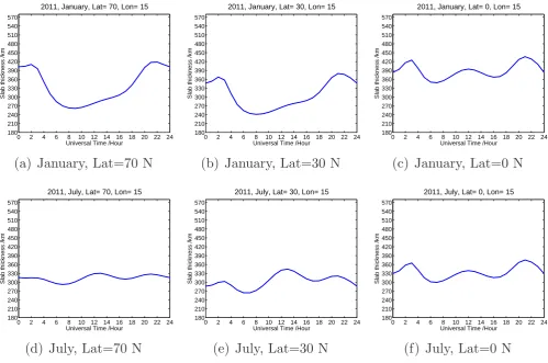
Figure 3 shows the mean diurnal variations of

τ

for the summer month July and the

winter month January during 2011 for low-, mid- and high-latitude locations. During

the winter month the slab thickness values range between about 250 km and 430 km

for high-latitude, 240 km and 350 km for mid-latitude and 340 km and 450 km for low

latitude location. In July the values are between 250 km and 370 km. For the

mid-and low-latitudes

τ

values seems to increase toward the equator. We observe two

ap-parent peaks during the pre-midnight and pre-sunrise periods for the winter period for

all three latitudes. Occurrence of similar pre-sunrise and post-sunset peaks in

τ

is

re-ported by many investigators for different latitude regions (cf. [Davies and Liu, 1991],

[Jayachandran et al., 2004], [Chuo, 2007], [Miro et al., 1999]). The pre-sunrise peak of

our modeled slab thickness is more pronounced during the winter period, in

agree-ment with results of the agree-mentioned papers. The night-time values of modeled

τ

are

higher compared to the day-time values during the winter month for all three

lati-tudes. During July this relation seems to be true just for the low latitude. During

so-lar minimum phases many observation based investigations (cf. [Jakowski et al., 1981],

[Jayachandran et al., 2004], [Chuo, 2007], [Stankov and Warnant, 2009]) generally

char-acterize the mean diurnal variations of the slab thickness by night-time values that are

substantially higher than the day-time values during different seasons for different

lat-itude locations except during the summer season for high- and mid-latlat-itudes.

0 2 4 6 8 10 12 14 16 18 20 22 24

180 210 240 270 300 330 360 390 420 450 480 510 540 570

Universal Time /Hour

Slab thickness /km

2011, January, Lat= 70, Lon= 15

(a) January, Lat=70 N

0 2 4 6 8 10 12 14 16 18 20 22 24

180 210 240 270 300 330 360 390 420 450 480 510 540 570

Slab thickness /km

(b) January, Lat=30 N

0 2 4 6 8 10 12 14 16 18 20 22 24

180 210 240 270 300 330 360 390 420 450 480 510 540 570

Slab thickness /km

(c) January, Lat=0 N

0 2 4 6 8 10 12 14 16 18 20 22 24

180 210 240 270 300 330 360 390 420 450 480 510 540 570

Slab thickness /km

2011, July, Lat= 70, Lon= 15

(d) July, Lat=70 N

0 2 4 6 8 10 12 14 16 18 20 22 24

180 210 240 270 300 330 360 390 420 450 480 510 540 570

Slab thickness /km

2011, July, Lat= 30, Lon= 15

(e) July, Lat=30 N

0 2 4 6 8 10 12 14 16 18 20 22 24

180 210 240 270 300 330 360 390 420 450 480 510 540 570

Slab thickness /km

2011, July, Lat= 0, Lon= 15

(f) July, Lat=0 N

Figure 3: Variation of slab thickness, 2011.

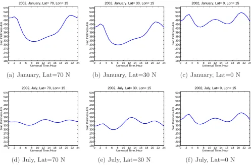
Figure 4 represents the mean diurnal variation of the slab thickness for January and

July during solar maximum year 2002 again for the low-, mid- and high-latitude

[image:5.595.48.548.61.392.2]

loca-8

Fig. 3. Variation of slab thickness, 2011.

show the mean diurnal and seasonal variations and effects of solar activity on the modeledτ values for low, middle and high latitudes. To calculate the modeledτ values we choose the months July and January of 2002 (a year of high solar activity) and July and January 2011 (low to medium solar activity). The solar radio flux index F10.7 ranges between 70 and 90 units (1 flux unit = 10−22W m−2Hz) in January 2011 and between 85 and 125 units in July 2011. For 2002 the F10.7 values are between 180 and 255 units in January and between 130 and 250 units in July.

To modelτ we calculate the values of TEC and NmF2 by means of the models NTCM-GL and NPDM, respectively. The calculations are made for the latitudes 0, 30 and 70 de-grees north at 15 dede-grees east longitude. The latitudes 0◦N, 30◦N and 70◦N are chosen to cover low-, mid- and high-latitude regions. The longitude of 15 degrees east is chosen to make the considered slab thickness results comparable to the results of the NmF2 validation performed in Sect. 5. Note that the most ionosonde stations considered in Sect. 5 are lo-cated around 15 degrees east of longitude. Since slab thick-ness modeling is just an interim result within this work, the consideration of the slab thickness results for any other lon-gitudes is not included in this paper. In the next step we em-ploy modeled TECmodand NmF2modto calculate slab

thick-ness according to the relation given by the Eq. (5). The slab thickness values are calculated every 60 min and afterwards averaged over the month.

Figure 3 shows the mean diurnal variations ofτ for the summer month July and the winter month January during 2011 for low-, mid- and high-latitude locations. During the winter month the slab thickness values range between about 250 and 430 km for high-latitude, 240 and 350 km for mid-latitude and 340 and 450 km for low-mid-latitude location. In July the values are between 250 and 370 km. For the mid- and low-latitudes, τ values seems to increase toward the equa-tor. We observe two apparent peaks during the pre-midnight and pre-sunrise periods for the winter period for all three latitudes. Occurrence of similar pre-sunrise and post-sunset peaks in τ is reported by many investigators for different latitude regions (cf. Davies and Liu, 1991; Jayachandran et al., 2004; Chuo, 2007; Miro et al., 1999). The pre-sunrise peak of our modeled slab thickness is more pronounced dur-ing the winter period, in agreement with results of the men-tioned papers. The nighttime values of modeledτ are higher compared to the daytime values during the winter month for all three latitudes. During July this relation seems to be true just for the low latitude. During solar minimum phases many observation-based investigations (cf. Jakowski et al., 1981;

(6)

0 2 4 6 8 10 12 14 16 18 20 22 24

180 210 240 270 300 330 360 390 420 450 480 510 540 570

Slab thickness /km

(a) January, Lat=70 N

0 2 4 6 8 10 12 14 16 18 20 22 24

180 210 240 270 300 330 360 390 420 450 480 510 540 570

Slab thickness /km

(b) January, Lat=30 N

0 2 4 6 8 10 12 14 16 18 20 22 24

180 210 240 270 300 330 360 390 420 450 480 510 540 570

Slab thickness /km

(c) January, Lat=0 N

0 2 4 6 8 10 12 14 16 18 20 22 24

180 210 240 270 300 330 360 390 420 450 480 510 540 570

Slab thickness /km

2002, July, Lat= 70, Lon= 15

(d) July, Lat=70 N

0 2 4 6 8 10 12 14 16 18 20 22 24

180 210 240 270 300 330 360 390 420 450 480 510 540 570

Slab thickness /km

2002, July, Lat= 30, Lon= 15

(e) July, Lat=30 N

0 2 4 6 8 10 12 14 16 18 20 22 24

180 210 240 270 300 330 360 390 420 450 480 510 540 570

Slab thickness /km

2002, July, Lat= 0, Lon= 15

(f) July, Lat=0 N

Figure 4: Variation of slab thickness, 2002.

tions. We observe that the solar phase change has influenced the increase of

τ

values on

all three latitudes for both summer and winter months. But for July the increasing is

much more smaller than for the winter month. The slab thickness values range between

320 km and 530 km for high-latitude, 300 and 470 km for mid-latitude and 430 km and

540 km for low latitude location during January. During July

τ

values are between 330

km and 380 km, 300 and 400 km and 340 and 420 km for high-, mid- and low-latitude

locations respectively. The increasing agree qualitatively with published results based

on long-time observations of

T EC

and

f oF

2 (cf. [Jayachandran et al., 2004]).

Concluding we can say that our modeling results are comparable with other model and

observation based investigations mentioned above.

5 Validation of the reconstructed

N mF

2 maps

To test the proposed

N mF

2 reconstruction algorithm we make a comparison between

the reconstructed

N mF

2

rec

values and ionosonde data,

N mF

2

IS

, first and modeled

N mF

2

mod

values and ionosonde data second. For validation the ionosonde stations

data of one-month period, particularly July 2011 is chosen. The data are selected at

different latitudes in the northern hemisphere around two longitudes 15 E and 130 E.

Figure 5 presents the variation of the solar radio flux index

F

10 .

7 in flux units for July

2011. As mentioned before the

F

10 .

7 index is a measure of the solar activity. The

[image:6.595.48.546.61.389.2]

F

10 .

7 data are obtained from the Space Physics Interactive Data Resource (SPIDR) of

NOAA’s National Geophysical Data Center (http://spidr.ngdc.noaa.gov/spidr/). As

Fig. 4. Variation of slab thickness, 2002.

Jayachandran et al., 2004; Chuo, 2007; Stankov and War-nant, 2009) generally characterize the mean diurnal varia-tions of the slab thickness by nighttime values that are sub-stantially higher than the daytime values during different sea-sons for different latitude locations except during the summer season for high and mid-latitudes.

Figure 4 represents the mean diurnal variation of the slab thickness for January and July during the solar maximum year 2002 again for the low-, mid- and high-latitude loca-tions. We observe that the solar phase change has influenced the increase ofτ values on all three latitudes for both sum-mer and winter months. But for July the increase is much smaller than for the winter month. The slab thickness values range between 320 and 530 km for the high-latitude, 300 and 470 km for the mid-latitude and 430 and 540 km for the low-latitude location during January. During Julyτvalues are be-tween 330 and 380 km, 300 and 400 km and 340 and 420 km for high-, mid- and low-latitude locations, respectively. The increase agrees qualitatively with published results based on long-time observations of TEC and foF2 (cf. Jayachandran et al., 2004).

In conclusion we can say that our modeling results are comparable with other model- and observation-based inves-tigations mentioned above.

5 Validation of the reconstructed NmF2 maps

To test the proposed NmF2 reconstruction algorithm we make a comparison between the reconstructed NmF2rec

values and ionosonde data, NmF2IS, first and modeled

NmF2mod values and ionosonde data second. For validation

the ionosonde stations’ data of a one-month period, specifi-cally July 2011, is chosen. The data are selected at different latitudes in the Northern Hemisphere around two longitudes: 15◦E and 130◦E.

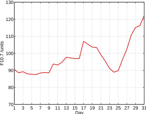
Figure 5 presents the variation of the solar radio flux index F10.7 in flux units for July 2011. As mentioned before, the F10.7 index is a measure of the solar activity. The F10.7 data are obtained from the Space Physics Interactive Data Re-source (SPIDR) of NOAA’s National Geophysical Data Cen-ter (http://spidr.ngdc.noaa.gov/spidr/). As can be observed in Fig. 5 the validation period contains days with middle and low solar activity. The global planetary 3 h index Kp varies between 0 and 5 units; thus also the geomagnetic activity is low to middle. Please note that the Kp index is given here just as a measure for the geomagnetic activity. It is not an input parameter for the NPDM model.

As a reference data set we used ionosonde data from the stations Tromsø, Juliusruh, Rome, Gibilmanna, Magadan,

(7)

1 3 5 7 9 11 13 15 17 19 21 23 25 27 29 31 70

80 90 100 110 120 130

Day

[image:7.595.50.284.63.246.2]

F10.7 /units

Fig. 5. The F10.7 (solar radio flux) index for July 2011.

I-Cheon and Okinawa. The ionosonde data are obtained from the National Geophysical Data Center. Table 1 shows the list of all used ionosonde stations with geographical locations.

First of all, the ionosonde data are filtered by a plausibility check. The plausibility check algorithm sorts out the values above 1013m−3or under 1010m−3if the corresponding mea-sured TEC values were neither unexpectedly high nor low. In parallel to this the NmF2 values are calculated applying both the NPDM Model and the reconstruction algorithm for the ionosonde station locations and time steps of availability of the ionosonde measurements.

The histograms of the NmF2 model residuals, NmF2IS−

NmF2mod, and reconstruction residuals, NmF2IS−NmF2rec,

are shown in Fig. 6. The left-side picture presents the his-togram of the reconstruction residuals as well as the corre-sponding mean, root mean square (rms) and standard devia-tion, and the right one the model residuals histogram. We can see that the residuals are normally distributed with a mean value of−2.4×1010for the reconstruction and 4.2×1010for the model residuals. The standard deviations are 13×1010 and the rms deviation is 13.2×1010 for the reconstruction and 13.7×1010for the model.

To get a first impression on the reconstruction results un-der disturbed conditions, we compare the reconstructed and modeled NmF2 values with ionosonde data for a day with a F10.7 jump and a day with stabile and low solar activ-ity during the validation period July 2011. As can be seen in Fig. 5 we have a local F10.7 peak on 17 July 2011; thus this day is selected. As a quiet day we choose 8 July 2011, because the F10.7 values during some days around 8 July stay nearly constant. As a reference data set we use again the ionosonde data from the stations Tromsø, Juliusruh, Rome, Gibilmanna, Magadan, I-Cheon and Okinawa. The residuals are calculated in the same way as described above. Figure 7 shows the histograms of the model and reconstruction

resid-Table 1. Ionosonde stations used for the validation.

Code Name Country Latitude Longitude TR170 Tromsø Norway 69.6◦N 19.2◦E JR055 Juliusruh Germany 54.6◦N 13.4◦E RO041 Rome Italy 41.8◦N 12.5◦E GM037 Gibilmanna Italy 37.6◦N 14◦E MG560 Magadan Russia 60◦N 151◦E IC437 I-Cheon South Korea 37.1◦N 127.5◦E OK426 Okinawa Japan 26.3◦N 127.8◦E

uals for the two picked-out days: 17 July 2011 (panels a and b) and 8 July 2011 (panels c and d).

We can observe that the values of the residual distributions for 8 July are nearly equal to the corresponding values calcu-lated for the whole month (cf. Fig. 6) for both reconstructed and model residuals. However, for 17 July the picture of the residual distribution values is significantly changed. The mean of the model residuals increases from 4.2×1010 aver-aged over the whole of July to 7.3×1010for 17 July, while the mean value of the reconstruction residuals decreases to 0.6×1010. Thus, for this day with a F10.7 peak we observe an improvement of the mean residuals by a factor of 12.17, com-paring the reconstruction and the model. The standard devi-ation is slightly increased for both reconstruction and model residuals, which is not unexpected for disturbed conditions. Due to the fact that within the reconstruction not only the F10.7 value but also actual TEC measurements are used, we expect that for periods of high solar activity and also during solar storms the reconstruction provides much more accurate results than the model. The next step will be to compare the reconstructed and modeled NmF2 values with measurements for a time period with high solar activity.

In conclusion we can say that both the model and the re-construction approach provide similar good results, but the reconstruction has a factor of 1.75 better mean value for the observed period with low to middle solar activity. It should be noted that the results and the quality of this reconstruc-tion approach strongly depend on the model slab thickness values. And these values essentially depend on the quality of the TEC and NmF2 models and on the condition that these two models fit together.

6 Conclusions

This paper presents the reconstruction approach for the F2 layer peak electron density. The main input for the recon-struction procedure is the TEC maps calculated from ground-based GNSS measurements. The algorithm can be run on a global or a local grid. The spatial resolution can be easily modified.

Currently the algorithm is used for routine generation of global NmF2 maps with spatial resolution of 2.5◦ latitude,

[image:7.595.308.549.82.181.2]

(8)

−0.8 −0.6 −0.4 −0.20 0 0.2 0.4 0.6 0.8 1 1.2

500 1000 1500 2000 2500 3000 3500

Electron density /1012m−3

Samples

Mean = −0.024 RMS = 0.132 STD = 0.130

(a)N mF₂I S₋N mF2rec

−0.8 −0.6 −0.4 −0.20 0 0.2 0.4 0.6 0.8 1 1.2

500 1000 1500 2000 2500 3000 3500

Samples

Mean = 0.042 RMS = 0.137 STD = 0.130

(b)N mF₂I S₋N mF2mod

Figure 6: Histograms of the residuals, July, 2011. Reconstruction residuals are on the

left side and model residuals on the right.

mean, RMS and standard deviation and the right one the model residuals histogram.

We can see that the residuals are normally distributed with mean value of

−

2 .

4 ×

10

for the reconstruction and 4

.

2 ×

10

for the model residuals. The standard deviations

are 13

×

10

and the RMS deviation is 13

.

2 ×

10

for the reconstruction and 13

.

7 ×

10

for the model.

To get a first impression on the reconstruction results under disturbed conditions, we

compare the reconstructed and modeled

N mF

2 values with ionosonde data for a day

with a F10.7-jump and a day with stabile and low solar activity during the

valida-tion period July 2011. As can be seen in Figure 5 we have a local F10.7-peak on

17/07/2011, thus this day is selected. As a quiet day we choose 08/07/2011, because

the

F

10 .

7 values during some days around the 8th of July stay nearly constant. As

reference data set we use again the ionosonde data from the stations Tromsø, Juliusruh,

Rome, Gibilmanna, Magadan, I-Cheon and Okinawa. The residuals are calculated in

the same way as described above. Figure 7 shows the histograms of the model and

reconstruction residuals for the two picked out days 17/07/2011 (sub-figures a) and b))

and 08/07/2011 (sub-figures c) and d)).

We can observe that the values of the residual distributions for the 8th of July are

nearly equal to the corresponding values calculated for the whole month (cf. Figure

6) for both reconstructed and model residuals. Whereas, for the 17th of July the

pic-ture of the residual distribution values is significantly changed. The mean of the model

residuals increases from 4

.

2 ×

10

averaged over the whole July to 7

.

3 ×

10

for the 17th

July, while the mean value of the reconstruction residuals decrease to 0

.

6 ×

10

. Thus,

for this day with a

F

10 .

7-peak we observe an improvement of the mean residuals by a

factor 12.17 comparing the reconstruction and the model. The standard deviation is

slightly increased for both reconstruction and model residuals, which is not unexpected

for disturbed conditions. Due to the fact, that within the reconstruction not only the

F

10 .

7 value but also actual

T EC

measurements are used, we expect that for periods of

high solar activity and also during solar storms the reconstruction provides much more

[image:8.595.101.495.61.224.2]

11

Fig. 6. Histograms of the residuals, July 2011. Reconstruction residuals are on the left side and model residuals on the right.

−0.8 −0.6 −0.4 −0.20 0 0.2 0.4 0.6 0.8 1 1.2

50 100 150

Samples

Mean = 0.006 RMS = 0.135 STD = 0.135

(a) N mF₂_{I S}₋N mF₂_rec_{, 17/07/2011}

−0.8 −0.6 −0.4 −0.20 0 0.2 0.4 0.6 0.8 1 1.2

50 100 150

Samples

Mean = 0.073 RMS = 0.153 STD = 0.135

(b) N mF₂_{I S}₋N mF₂_mod_{, 17/07/2011}

−0.8 −0.6 −0.4 −0.20 0 0.2 0.4 0.6 0.8 1 1.2

50 100 150

Samples

Mean = −0.021 RMS = 0.133 STD = 0.132

(c) N mF₂_{I S}₋N mF₂_rec_{, 08/07/2011}

−0.8 −0.6 −0.4 −0.20 0 0.2 0.4 0.6 0.8 1 1.2

50 100 150

Samples

Mean = 0.048 RMS = 0.110 STD = 0.099

(d) N mF₂_{I S}₋N mF₂_mod_{, 08/07/2011}

Figure 7: Histograms of the reconstruction residuals (left side) and model residuals

(right side).

Fig. 7. Histograms of the reconstruction residuals (left side) and model residuals (right side).

5◦longitude and time resolution of 5 min. The reconstructed electron density maps are offered to users via the opera-tional data service SWACI (http://swaciweb.dlr.de) at DLR Neustrelitz.

The presented reconstruction method provides the users the possibility to get an improved picture of the actual

iono-sphere. They are fast and easy in application and suitable for the operational service. Comparing the NmF2 reconstruction and NPDM model with ionosonde data an improvement of the mean residuals by a factor 1.75 have been observed. For the standard and rms deviations we get similar results.

(9)

Our next steps will be to validate the presented reconstruc-tion method under different solar and geomagnetic activity conditions and to improve the method by assimilation of the ionosonde measurements.

Acknowledgements. The authors thank the IGS for making

avail-able high-quality GPS observation data. The authors are also grate-ful to NGDC for disseminating ionosonde data via SPIDR. Many thanks also to the reviewers of the manuscript for very helpful com-ments.

The service charges for this open access publication have been covered by a Research Centre of the Helmholtz Association.

Topical Editor K. Kauristie thanks two anonymous referees for their help in evaluating this paper.

References

Angling, M. J. and Cannon, P. S.: Assimilation of radio occultation measurements into background ionospheric models, Radio Sci., 39, RS1S08, doi:10.1029/2002RS002819, 2004.

Angling, M. J. and Khattatov, B.: Comparative study of two as-similative models of the ionosphere, Radio Sci., 41, RS5S20, doi:10.1029/2005RS003372, 2006.

Bust, G. S., Garner, T. W., and Gaussiran II, T. L.: Ionospheric Data Assimilation Three-Dimensional (IDA3D): A global, multisen-sor, electron density specification algorithm, J. Geophys. Res., 109, A11312, doi:10.1029/2003JA010234, 2004.

Bust, G. S. and Mitchell, C. N.: History, current state, and future directions of ionospheric imaging, Reviews of Geoph., 46, 23 pp., 2008.

Chuo, Y. J.: The variation of ionospheric slab thickness over equa-torial ionization area crest region, J. Atmos. Terr. Phys., 69, 947– 954, 2007.

Davies, K.: Ionospheric Radio, Peter Peregrinus Ltd, London, 1990. Davies, K. and Liu, X. M.: Ionospheric slab thickness in middle and

low latitudes, Radio Sci., 26, 997–1005, 1991.

Hern´andez-Pajares, M., Juan, J. M., Sanz, J., Orus, R., Garcia-Rigo, A., Feltens, J., Komjathy, A., Schaer, S. C., and Krankowski, A.: The IGS VTEC maps: a reliable source of ionospheric informa-tion since 1998, J. Geod., 83, 263–275, doi:10.1007/s00190-008-0266-1, 2009.

Hoque, M. M. and Jakowski, N.: Estimate of higher order iono-spheric errors in GNSS positioning, Radio Sci., 43, RS5008, doi:10.1029/2007RS003817, 2008.

Hoque, M. M. and Jakowski, N.: A new global empirical NmF2 model for operational use in radio systems, Radio Sci., 46, RS6015, doi:10.1029/2011RS004807, 2011.

Huang, Y.-N.: Some results of ionospheric slab thickness observa-tions at Lunping, J. Geophys. Res., 88, 5517–5522, 1983. Jakowski, N., Bettac, H. D., Lazo, B., and Lois, L.: Seasonal

varia-tions of the columnar electron content of the ionosphere observed in Havana from July 1974 to April 1975, J. Atmos. Terrestrial Phys., 43, 7–11, 1981.

Jakowski, N., Putz, E., and Spalla, P.: Ionospheric storm character-istics deduced from satellite radio beacon observations at three European stations, Ann. Geophys. 8, 343–352, 1990.

Jakowski, N., Mielich, J., Hoque, M. M., and Danielides, M.: Equiv-alent slab thickness at the mid-latitude ionosphere during solar cycle 23, 38th COSPAR Scientific Assembly, 18–25 July 2010, Bremen, Germany, 2010.

Jakowski, N., Hoque, M. M., and Mayer, C.: A new global TEC model for estimating transionospheric radio wave propagation errors, J. Geod., 85, 965–974, doi:10.1007/s00190-011-0455-1, 2011a.

Jakowski, N., Mayer, C., Hoque, M. M., and Wilken, V.: Total Elec-tron Content Models And Their Use In Ionosphere Monitoring, Radio Sci., 46, RS0D18, doi:10.1029/2010RS004620, 2011b. Jayachandran, B., Krishnankutty, T. N., and Gulyaeva, T. L.:

Clima-tology of ionospheric slab thickness, Ann. Geophys., 22, 25–33, doi:10.5194/angeo-22-25-2004, 2004.

Kersley, L. and Hajeb-Hosseinieh, H.: The dependence of iono-spheric slab thickness on geomagnetic activity, J. Atmos. Terr. Phys., 38, 1357–1360, 1976.

Leitinger, R., Ciraolo, L., Kersley, L., Kouris, S. S., and Spalla, P.: Relations between electron content and peak density-regular and extreme behaviour, Ann. Geophys. Suppl., 47, 179–194, 2004. Miro, G., Jakowski, N., and de la Morena, B. A.: Equivalent

Slab Thickness of the Ionosphere in Middle Latitudes Based on TEC/f0F2 Observations Over EL Arenosillo, in: Proc. 3rd COST251 Workshop, edited by: Hanbaba, R. and de la Morena, B. A., September, 1998, 87–92, 1999.

Nava, B., Coisson, P., and Radicella, S. M.: A new version of the NeQuick ionosphere electron density model, J. Atmos. So-lar Terr. Phys., 70, 1856–1862, doi:10.1016/j.jastp.2008.01.015, 2008.

Scherliess, L., Schunk, R. W., Sojka, J. J., and Thomp-son, D. C.: Development of a physics-based reduced state Kalman filter for the ionosphere, Radio Sci., 39, RS1S04, doi:10.1029/2002RS002797, 2004.

Stankov, S. M. and Jakowski, N.: Topside ionospheric scale height analysis and modeling based on radio occultation measurements, J. Atmos. Solar-Terr. Phys., 68, 134–162, 2006.

Stankov, S. M. and Warnant, R.: Ionospheric slab thickness – Analy-sis, modelling and monitoring, Adv. Space Res., 44, 1295–1303. Unglaub, C., Jacobi, Ch., Schmidtke, G., Nikutowski, B., and Brun-ner, R.: EUV-TEC proxy to describe ionospheric variability us-ing satellite-borne solar EUV measurements: First results, Adv. Space Res., 47, 1578–1584, 2011.