RO module RTD analyses based on directly processing conductivity signals

Journal of Membrane Science 306 (2007) 355–364

RO module RTD analyses based on directly processing

conductivity signals

Qingfeng Yang

, Alexander Drak

, David Hasson

, Raphael Semiat

a_{School of Environmental Science and Engineering, Shanghai Jiao Tong University,}

800 Dongchuan Road, Shanghai 200240, China

b_{GWRI Rabin Desalination Research Laboratory, Department of Chemical Engineering,}

Technion-Israel Institute of Technology, Haifa 32000, Israel

Received 9 April 2007; received in revised form 9 September 2007; accepted 14 September 2007 Available online 19 September 2007

Abstract

Residence time distribution (RTD) techniques can be used to diagnose the flow characteristics in spiral wound reverse osmosis (RO) modules. However, the methods of processing tracer response conductivity signals and mathematically modeling of RTD curves often involve complicated steps including conductivity-concentration transformation, baseline selection and the use of exit age distribution function ofEt, or dimensionless

exit age distribution function ofE_θ. In this paper, a simple and direct method for processing RTD signals from conductivity data was developed for spiral wound membrane RO system. Two models were tested: axial dispersion (AD) model and exponentially modified Gaussian (EMG) model. The results show that the present method provides a simple, fast and accurate RTD data reduction. The levels of the axial mixing intensities, characterized by the dispersion numberD/uL, indicated significant deviations from ideal plug flow in both the laboratory and the industrial size modules. In both the modules, the dispersion coefficientDincreased roughly linearly with the Reynolds number. Membrane fouling and worn-out led to an increase inD. Moreover, the values of mean residence time ¯_tandD/uLobtained from the EMG model were more stable against the change of the curve tail length, especially for the parameterD/uL. Furthermore, RTD analysis also indicated that the membrane wearing-out could lead to dead zones.

© 2007 Elsevier B.V. All rights reserved.

Keywords: Spiral wound module; Reverse osmosis; Residence time distribution

1. Introduction

Reverse osmosis (RO) is widely applied in various fields such as desalination, raw water treatment and ultrapure water production. The design of the vast majority of RO plants is based on spiral wound membrane modules. Although spiral wound modules have an overall favorable performance, there is a wide scope for improving their flow performance and thereby lowering costs. Improved module design could be achieved by better understanding the geometric and operating parameters that determine the complex flow patterns occurring in a spiral wound module.

∗_{Corresponding author. Tel.: +86 21 54748942; fax: +86 21 54748942.}

E-mail address:[email protected](Q. Yang).

Residence time distribution (RTD) techniques have long been recognized in the chemical industry to be powerful tools for characterizing flow patterns and diagnosing malfunctioning in complex flow equipment such as packed bed catalytic reactors [1]. The basic principle of the technique is to inject a tracer material, such as a dye, a conductive solution or a radioactive compound, in the form of a “pulse” or a “step change” and to determine the exit concentration of the tracer material. The shape of the “response signal” can be used to determine important flow parameters such as the mean residence time of the fluid in the equipment, the presence of dead volumes and/or bypass streams, as well as the intensity of mixing effects along radial and axial directions[1].

One of the main goals in the design of a spiral wound module is to ensure uniformity of flow of the feed as it enters from the space above the membrane roll into the feed flow passages of the membrane roll. In view of other conflicting design

iments[4–6]were evaluated by axial mixing intensities through fitting the data to two theoretical models: axial dispersion (AD) model and exponentially modified Gaussian (EMG) model. In the experiments, the RTD data were acquired by conductomet-ric measurement of the response to a NaCl pulse injected to the feed water. However, the tracer response signal processing involved complicated data reductions including conductivity-concentration transformation, baseline selection and the use of exit age distribution function ofEtor dimensionless exit age

dis-tribution function ofE_θ. In this paper, a simple and direct method for processing RTD signals from conductivity measurements was developed for spiral wound membrane RO system. RTD parameters such as mean residence time, dispersion number and dispersion coefficient were studied under various condi-tions. Furthermore, the effect of signal tail length on the RTD parameters and the dead volume in worn module were also discussed.

2. Theory

2.1. Direct calculation of RTD parameters from discrete experimental data

Since there is a linear relationship between solution conduc-tivitykiand solution concentrationCiof the tracer solution, the

concentration can be expressed as:

Ci=aki+b (1)

Thus, the mean residence time ¯tcan be obtained directly from conductivity signals according to the definition[1]:

¯ t=

ti(ki−k0)ti

(ki−k0)ti

(2)

and the variance is given by:

σ_t2=

t2_i(ki−k0)t_i

(ki−k0)t_i −

¯

t2 (3)

In the traditional method, the dimensionless functions ofE_θ, σ_θ2andθare usually used, as shown in following forms:

Eθ=

¯_t(ki−k0)

(ki−k0)t_i =

V

MC (4)

ule. For an ideal flow system approaching plug flow,D/uL→0. For a highly mixed flow system, D/uL→ ∞. The dispersion coefficientDrepresents the axial spreading process. Large D

means rapid spreading of the tracer curve, smallDmeans slow spreading andD= 0 means no spreading, or plug flow.

2.2. Axial dispersion model

RTD response curves in spiral wound membrane RO system can be fitted by axial dispersion (AD) model, which is given in dimensionless groups[1]:

Eθ =

1 √

4π(D/uL) exp

− (1−θ)2 4θ(D/uL)

(8)

By combining Eqs.(1),(4),(5)and(8), the following relation-ship between conductivity and time can be obtained:

k= √ M/aV 4π(D/uL) exp

− (1−t/¯t)2 4t/¯_t(D/uL)

−b

a (9)

Thus, through curve fit according to the above equation, the RTD parameters of ¯t,D/uLandDcan be obtained directly from conductivity signals. The curve fit can be performed by non-linear fit using Origin software with appropriate initial parameter values.

2.3. Exponentially modified Gaussian model

A more accurate model, exponentially modified Gaussian (EMG) model, can be used for RTD signals. The EMG model has been widely used to model chromatographic peaks[7]. It is a convolution of a Gaussian and an exponential decay function, and usually to describe peaks with asymmetrical zone broaden-ing to the rear. The form of this equation is[8]:

C(t)= A 2t0

exp

w2 2t20

−t−xc

t0

×

erf t√−xc 2w − w √ 2t0 +1 (10)

whereA,xc,w,t0are model parameters. The mean residence

Fig. 1. Experimental set-up (C, conductivity; P, pressure; F, flow rate).

By combining Eqs. (1) and (10), the expression between conductivity and time can be gained:

k(t)= A 2t0a

exp

w2 2t02

−t−xc

t0

×

erf t√−xc 2w −

w √

2t0

+1

−b

a (11)

Thus, through curve fit according to the above equation, the mean residence time can also be obtained directly from conductivity signals. The curve fit can also be carried out by the GaussMod function using Origin software. Because the Gaussmod function is the internal fit function in Origin, it does not need to set the initial parameter values by using a quick-fit Origin C file, which was very convenient to get the RTD parameters.

3. Experimental

The residence time distribution was measured by injecting a concentrated NaCl solution at the inlet of the membrane mod-ule, and monitoring the response at its outlet with a conductivity probe.Fig. 1demonstrates the schematic flowchart of the sys-tem. The system consists of the following elements: membrane unit, feed vessel, centrifugal pump, heat exchanger, air pressure vessel and solution pressure vessel.

Pressurized tap water was supplied to the module by a cen-trifugal pump. A batch of concentrated NaCl solution was injected from a solution pressure vessel and pressurized by com-pressed air over the solution. A NaCl pulse was introduced into the module, when the ball valve connected to the inlet pipe of the spiral module was opened. The response of the NaCl tracer solution in the concentrate channel was monitored using a conductivity meter (model 759II-131-4A-45, MYRON L Company, USA), which has a response time of the order of milliseconds.

Two types of spiral wound RO modules were employed to carry out RTD experiments: small laboratory size and indus-trial size modules. The small module is FilmTEC TW30-2514, supplied by DOW Chemical Company. The module parameters are: length 35.56 cm (14 in.), diameter 6.35 cm (2.5 in.), 2 sheets, 0.687 m2. The industrial modules are two 20-cm (8-in.)

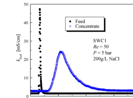
diam-Fig. 2. Typical RTD response signals obtained by injection a pulse of 200 g/L NaCl solution.

eter modules: one worn and one new. The membrane type is SWC1, manufactured by Hydranautics. The module parameters are: length 101.6 cm (40 in.), diameter 20 cm (8 in.), 17 sheets, 28.7 m2.

The small spiral wound module was operated at 10–20 bar and feed water flow rates in the range of 210–940 L/h, corre-sponding to Reynolds numbers (Re) of 60–240. The industrial size spiral wound module was operated at 10–40 bar and feed water flow rates in the range of 1–10 m3/h, corresponding toRe

of 60–370. In order to realize the pulse injection, the volume of the injected NaCl solution was small and was about 100 mL. The relatively high NaCl concentrations of 10 and 200 g/L were adopted for the small TW30-2512 and big SWC1 modules, respectively, which ensures an obviously detectable response signals considering the dilution effect by the high flow rates of feed water.

The Reynolds number for flow in a spiral wound module is defined by[2]:

Re=ρdhu

μ (12)

and the hydraulic diameterdhis defined as:

dh= 4ε

(2/ h)+(1−ε)SV,SP

(13)

The flow rate in the concentrate channel is defined as:

Qfc=Qf+Qc

2 =Qc+ Qp

2 (14)

4. Results and discussion

4.1. Typical RTD response signal

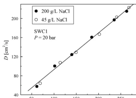
Fig. 3. Effect of injected NaCl concentration on dispersion coefficient.

that the NaCl concentration decreased from 200 to 30 g/L (feed conductivity 47.5 mS/cm inFig. 2), corresponding to a decrease in osmotic pressure from 160 to 24 bar. This result indicates the obvious dilution effect by the high feed water flow rate. The RTD response signal detected by the conductivity meter at the outlet of the membrane module indicates that the maximum conduc-tivity was 3.5 mS/cm, corresponding to an osmotic pressure of 1.4 bar. As a result, the concentration of 200 g/L NaCl greatly diminished in the membrane module, leading to a very small localized possible reverse flow through membrane. The direct experimental evidence is also shown inFig. 3. By using 200 and 45 g/L NaCl as injected solutions, which corresponds to osmotic pressures of 24 and 6 bar measured by the conductivity meter prior to the membrane module, the measured dispersion coeffi-cients had the same value at a feed pressure of 20 bar. The above results show that the adopted NaCl concentration of 200 g/L has no effect on the flow dispersion in the membrane module since the injected volume is very small.

The section of the housing prior to the element is short, and the corresponding Re is high and ranges between 5000 and 20,000. Therefore, the stagnant region in the housing prior

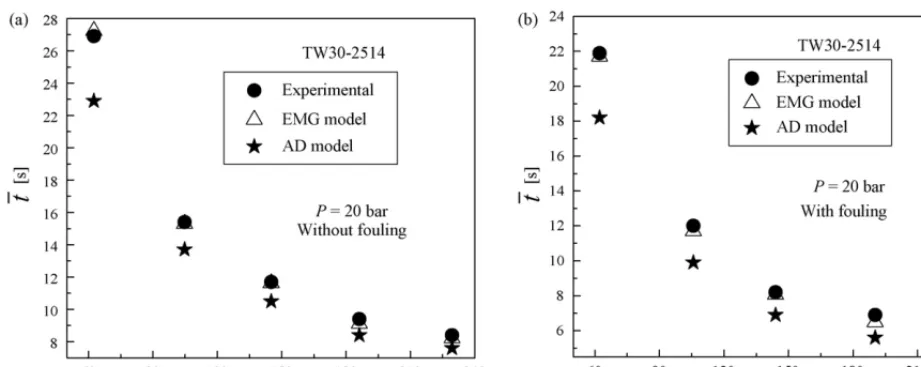
they are 11.7, 10.5 and 11.6 s from the experimental data, AD model and EMG model, respectively. The errors for the AD and EMG models are 10.3 and 0.6%, respectively.

By using the TW30-2514 small module with fouling, the values of ¯tobtained from the experimental data, AD model and EMG model are 8.2, 7.0 and 8.1 s, respectively, as shown in Fig. 4b. The errors for the AD and EMG models are 14.6 and 1.2%, respectively. FromFig. 4, it can be seen that EMG model behaves better in data fit.

The change of ¯t with Re, obtained from direct processing of conductivity signals, is given inFig. 5. It can be seen that ¯

t becomes shorter with the increase in Re. The values of ¯t extracted from the EMG model are almost identical to those measured from the experiments, while there are big differ-ences between the values from the experiments and AD model. However, the differences decrease with the increase of Re. Compared to the results in the absence of fouling, the mean res-idence time in the presence of fouling is shorter under identical conditions.

In the axial dispersion model (dispersed plug flow model), the fluctuations of velocity profile are due to different flow velocities and to molecular and turbulent diffusions. The model implies that there exist no stagnant pockets and no gross bypassing or short-circuiting of fluid in the vessel[1]. However, for spiral wound RO modules, it is difficult to eliminate stagnant regions

Fig. 5. (a) Change of mean residence time withRefor the TW30-2514 small module without fouling. (b) Change of mean residence time withRefor the TW30-2514 small module with fouling.

and there may exist dead volumes in the concentrate channel [2,9–11]. This may be one of the reasons for the error in fitting RTD curves using the AD model.

Fig. 6a shows the effect of Re on the dispersion number

D/uL at the feed pressure of 20 bar according to the EMG model. It can be seen that the D/uL tends to decrease with the increase in Re, which means that the flow distribution improved with increasing Re. In the presence of fouling, the values ofD/uLare greater than those in the absence of foul-ing, indicating that the flow distribution worsened. Thus, the fouling deposit increased the non-uniformity of the flow dis-tribution. The presence of a fouling deposit was also found to increase the dispersion coefficient, as shown in Fig. 6b. Dis-persion coefficients for the clean membrane (D= 6–10 cm2/s at

Re= 62–230) increased toD= 7–20 cm2/s atRe= 62–230 in the presence a fouling layer. After fouling, the smooth membrane surface would become rough, which could increase the flow resistance and result in fluid backmixing. Thus, the presence of fouling in the membrane channel augments the axial dispersion extent.

Fouling deposit increases the deviation from plug flow, result-ing in a more severe dispersed flow. Accordresult-ing to the analyses above, this will increase the deadlocks, thus reducing permeate flow rate and to enhancing local fouling process. Therefore, the fouling exerts a considerable effect on the flow dispersion and the membrane performance.

4.3. RTD tests for the new and worn SWC1 industrial modules

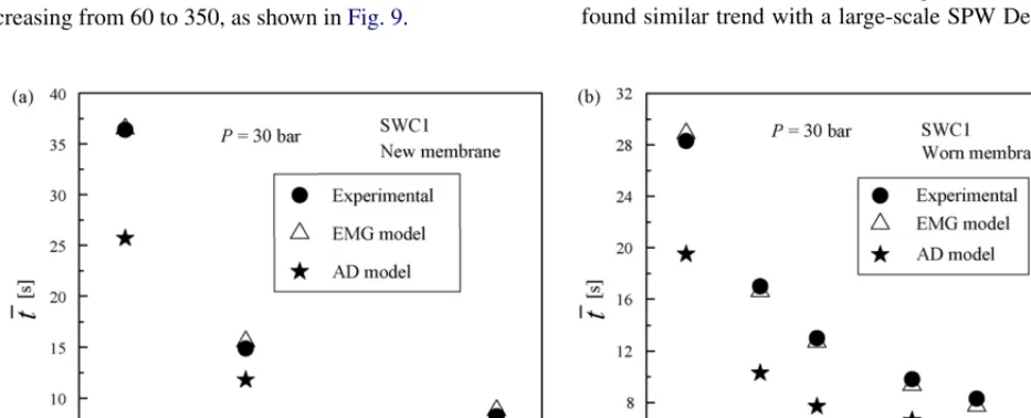
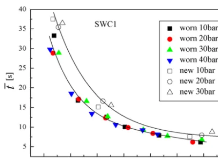
RTD test results are shown inFigs. 7 and 8by using the new and worn SWC1 industrial modules. It can be seen that under various conditions, based on the direct processing of conductiv-ity signals, the mean residence time can be successfully extracted from the experimental data, AD model and EMG model by using the Eqs.(2),(9)and(11). Furthermore, the mean residence times extracted from EMG model have almost the same values as those from the experimental data.

Under identical conditions, the mean residence time for the new SWC1 module is longer than the value for the worn SWC1

Fig. 7. (a) Result of RTD test by direct processing of conductivity signal for the new SWC1 industrial module. (b) Result of RTD tests by directly processing conductivity signal for the worn SWC1 industrial module.

module, just as demonstrated inFig. 8. This may be due to the channel structure change when the membrane module became worn.

4.4. Effect of feed pressure on RTD parameters

Conceivably, increase of feed pressure might exert some effect on the geometry of the flow passages and affect the flow characteristics. Accordingly, RTD experiments were carried out at the feed pressures over a range of 10–40 bar. However, the RTD data show that feed pressure had no effect at all on the magnitude of the dispersion coefficientD, indicating no distor-tion of the flow passages by a pressure increase, as shown in Figs. 9 and 10.

At different feed pressures, the mean residence time for the new SWC1 module is longer than the value for the worn SWC1 module. However, the difference decreases from 10 to 1 s with

Reincreasing from 60 to 350, as shown inFig. 9.

Dispersion coefficients for the new industrial size mem-brane illustrated inFig. 10a (D= 20–130 cm2/s atRe= 60–350) were higher than those for the new laboratory size mem-brane illustrated in Fig. 6b (D= 6–10 cm2/s at Re= 62–230). Dispersion coefficients for the worn industrial size membrane (D= 50–240 cm2/s at Re= 60–350) were significantly higher than those of the new membrane. Thus dispersion coefficient data could serve to characterize the degree of wear of a spiral wound module.

One of the main goals in the design of a spiral wound mod-ule is to ensure uniformity of the fluid flow in the channel. However, it is difficult to achieve a uniform flow distribution. Fig. 10b describes the effect ofReonD/uLat the feed pressure of 10–40 bar. It can be seen that theD/uLdecreases with increas-ingRe, which means that the flow distribution improved with increasingRe. This is consistent with the result obtained by the TW30-2514 module. Van Gauwbergen and Baeyens[11]also found similar trend with a large-scale SPW Desal 4040 11AG

Fig. 9. Effect of feed pressure on mean residence time for the SWC1 industrial modules.

membrane. An interesting result that may have practical impli-cations is that a worn membrane displays higherD/uLthan in a new membrane. Membrane wear seems to worsen the flow dis-tribution. The wear of a membrane thus could be characterized from RTD measurements.

From above results, it can be seen that the levels of the axial mixing intensities, characterized by the dispersion coefficient

D, indicated significant deviations from ideal plug flow in both the laboratory and the industrial size modules. In both systems, the dispersion coefficient increased roughly linearly with the Reynolds number, as shown inFigs. 6b and 10a.

4.5. Effect of tail length on¯_tand D/uL

From above RTD analyses, it can be seen that the EMG model provides an excellent fit for the RTD response data. Further-more, the RTD parameters extracted from the EMG model such as mean residence time ¯tand dispersion numberD/uLare more stable than those evaluated by the discrete experimental data when the curve tail length changes.Fig. 11a shows an original RTD curve obtained in a test for the new SWC1 module at a feed pressure of 20 bar and aReof 160. When the curve tail length

changed from 40 to 70 s, ¯tandD/uLwere calculated by the dis-crete experimental data and the EMG model, respectively. Four endpoints of the curve tail were selected and they are at 40, 50, 60 and 70 s. The results are shown inFig. 11b. It can be seen that the values of ¯t andD/uLobtained from the experimental data change with the change of the curve endpoint. The mean residence time increases from 16.5 to 17 s when the curve end-point changes from 40 to 70 s, leading to a small variation of 3%. However, the correspondingD/uLchanges from 0.047 to 0.067 when the curve endpoint changes from 40 to 70 s, leading to a large variation of 43%. It can be seen that the variation for

D/uLis larger than the one for ¯twhen they were evaluated by the discrete experimental data. Compared to the above results obtained from the experimental data, the values of ¯tandD/uL

extracted from the EMG model do not change with the curve tail length, as shown inFig. 11b. Therefore, the EMG model can give more stable RTD parameters, especially for the parameter

D/uL.

For the worn SWC1 module, similar results are also obtained. Figs. 12 and 13demonstrate the effect of the tail length on ¯tand

D/uLfor the worn SWC1 module at a feed pressure of 10 bar and

Reof 69 and 266, respectively. It can be seen that the parameters of ¯tandD/uLextracted from the EMG model are stable, while they change a lot with the curve tail length when they were calculated from the discrete experimental data. In Fig. 12b, ¯t evaluated from the experimental data changes from 31.1 to 33.9 s when the curve endpoint changes from 80 to 220 s, resulting in a small change of 9%. The correspondingD/uLchanges from 0.086 to 0.113, leading to a large variation of 31%. InFig. 13b, ¯

tevaluated from the experimental data changes from 8.3 to 8.6 s when the curve endpoint changes from 40 to 77 s, resulting in a small change of 4%. The correspondingD/uLchanges from 0.086 to 0.122, leading to a large variation of 42%. Thus, the EMG model can also give more stable RTD parameters for the worn module, especially for the parameterD/uL.

From the above results, it can be seen that it is important to develop models for RTD tests. Models are also useful for representing flow in real vessels, for scale-up, and for diagnosing poor flow[1].

Fig. 11. (a) RTD curve for the new SWC1 module. (b) Effect of the curve tail length on ¯tandD/uLfor the new SWC1 module.

Fig. 12. (a) RTD curve for the worn SWC1 module. (b) Effect of the curve tail length on ¯tandD/uLfor the worn SWC1 module.

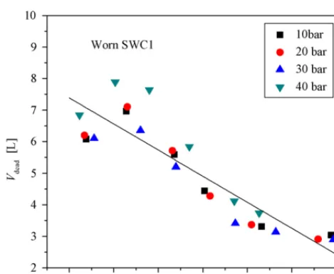
4.6. Change of dead volume with Reynolds number based on the directly processing conductivity data

The mean residence time of the fluid is an important char-acteristic of the spiral wound membrane module, and the dead volumes can be diagnosed by using the accurately calculated

values of the mean residence times.Fig. 14gives the change of the measured dead volume of concentrate channel withRein the worn SWC1 module. Supposing there is no dead volume in the new SWC1 module[6], the dead volume in the concentrate channel could be obtained by the product of two parameters: one is the fluid flow rate in the channel, and the other is the ¯t

Fig. 14. Effect ofReon the channel dead volume for the worn SWC1 industrial module.

difference between the values of the new and worn modules at the same Re. The mean distribution time ¯t was extracted from the EMG model and shown in Fig. 9. It can be seen that the measured concentrate channel dead volume gradually decreases with increasingRe. This may be due to the improve-ment in flow distribution with increasing Re, as illustrated in Fig. 10b.

For the worn module, the membrane surface became rough and also inevitably contained some fouling which was difficult to wash off completely. Thus, the flow resistance and fluid back-mixing would increase for the worn module. Consequently, the dead volume existed in the worn module. The above result indi-cates that the membrane wearing-out will lead to dead zones in the spiral wound module. The presence of dead zones in spiral wound membrane element both enhances local concentration polarization and reduces overall performance[12]. Van Gauw-bergen and Baeyens[11]also verified the existence of the dead volume in spiral wound RO module.

5. Conclusions

A simple and direct method for processing RTD signals from conductivity data was developed for spiral wound membrane RO system. Two models were tested: the simple AD model and the more elaborate EMG model. The results show that the present method provides a simple and fast RTD data reduction. The EMG mode could fit the RTD data much better than the AD mode. The levels of the axial mixing intensities, characterized by the dispersion numberD/uL, indicated significant deviations from ideal plug flow in both the laboratory and the industrial size modules. In both modules, the dispersion coefficientDincreased roughly linearly with the Reynolds number. Membrane fouling and worn-out led to an increase inD. Moreover, the values of mean residence time ¯tandD/uLobtained from the EMG model were more stable against the change of the curve tail length, especially for the parameterD/uL. The membrane wearing-out could lead to dead zones.

Acknowledgements

The financial support from the National Natural Science Foundation of China (Grant No. 20306015 and No. 20676077) is gratefully acknowledged.

Nomenclature

Ci concentration (kg/m3)

dh hydraulic diameter (m)

D dispersion coefficient

D/uL dispersion number

Et exit age distribution (s−1)

E_θ dimensionless exit age distribution

h membrane channel height (m)

ki conductivity (␮m/cm)

L module flow length (m)

M tracer mass (kg)

Qc outlet flow rate in the channel (L/h)

Qf inlet flow rate in the channel (L/h)

Qfc average flow rate in the channel (L/h)

SV,SP specific surface of the spacer (m−1)

t time (s) ¯

t mean residence time (s)

u average membrane flow velocity (m/s)

V module flow volume (m3)

Vdead dead volume (L)

Greek symbols

ε membrane channel porosity μ average solution viscosity (Pa s) θ dimensionless mean residence time ρ average solution density (kg/m3) σ_t2 variance

σ_θ2 dimensionless variance

References

[1] O. Levenspiel, Chemical Reaction Engineering, third ed., John Wiley, New York, 1999.

[2] D. Van Gauwbergen, J. Baeyens, Macroscopic fluid flow conditions in spiral wound membrane elements, Desalination 110 (1997) 287– 299.

[3] E. Roth, M. Kessler, B. Fabre, A. Accary, Sodium chloride stimulus-response experiments in spiral wound reverse osmosis membranes: a new method to detect fouling, Desalination 121 (1999) 183– 193.

[4] A. Drak, Q.F. Yang, D. Hasson, R. Semiat, Detection of spiral wound mod-ule defects by RTD analyses, in: Proc. IDA World Congress on Desalination and Water Reuse, Paper SP05-033, Singapore, 11–16 September, 2005, p. 20.

[5] D. Hasson, A. Drak, Q.F. Yang, R. Semiat, Effect of axial dispersion on the concentration polarization level in spiral wound modules, Desalination 199 (2006) 451–453.