On the influence of CMEs on the global 3-D coronal electron density

Ann. Geophys., 29, 1019–1028, 2011 www.ann-geophys.net/29/1019/2011/ doi:10.5194/angeo-29-1019-2011

© Author(s) 2011. CC Attribution 3.0 License.

Annales

Geophysicae

On the influence of CMEs on the global 3-D coronal electron density

M. Kramar1,2, J. Davila2, H. Xie1,2, and S. Antiochos2

1_{Physics Department, The Catholic University of America, 620 Michigan Ave NE, Washington, D.C. 20064, USA} 2_{NASA Goddard Space Flight Center, Greenbelt, MD 20771, USA}

Received: 11 June 2009 – Revised: 18 February 2011 – Accepted: 18 May 2011 – Published: 15 June 2011

Abstract. In order to analize the influence of a Coronal Mass Ejection (CME) on the coronal streamer belt, we made 3-D reconstructions of the electron density in the corona at he-liospheric distances from 1.5 to 4Rfor periods before and after a CME occured. The reconstructions were performed using a tomography technique. We studied two CME cases: (i) a slow CME on 1 June 2008; (ii) two fast CMEs on 31 December 2007 and 2 January 2008. For the first case of slow CME, it was found: (i) the potential magnetic field con-figuration in the CME initiation region before the CME does not agree with the coronal density structure while after the CME the agreement between the field and density is much better. This could be manifistation of that that the field was non-potential before the CME and after the CME the field relaxes towards a more potential state. (ii) It was shown that the dimming caused by the slow CME is not due to rotation of the corona and a line-of-sight (LOS) effect but a streamer blow out effect took place.

Keywords. Solar physics, astrophysics, and astronomy (Corona and transition region; Flares and mass ejections; Magnetic fields)

1 Introduction

Coronal Mass Ejections (CME) plays an important role for space weather research. There are still many open ques-tions connected with CME initiation, propagation and in-fluence on the ambient corona (Hudson et al., 2006; Mikic and Lee, 2006). Recent research has revealed, however, that CMEs involve the release of the magnetic energy stored in magnetic field (Forbes, 2000; Klimchuk, 2001). So, analyz-ing the magnetic field could help to understand the nature of

Correspondence to: M. Kramar ([email protected])

CMEs. But for the moment our knowledge about the coronal magnetic field is very limited. The direct Zeeman and Hanle effect (usually used for deriving the magnetic field at the pho-tosphere) measurements in the corona are very difficult due to much lower strength of the coronal magnetic field (about 1 Gauss (Lin et al., 2004)) and because of the high temper-ature of the coronal plasma. Moreover, the interpretation of such kind of measurements is not straightforward due to the fact that the corona is opticaly thin and these measurements are essentially line-of-sight (LOS) integrated. However the latest progress in these measurements (Lin et al., 2004; Tom-czyk et al., 2008; Judge, 2007) and the vector tomography technique (Kramar et al., 2006; Kramar and Inhester, 2007) gives a hope for increasing our knowledge about the coronal magnetic field.

Recently, vector magnetograms from the photosphere have became available, which in principle supply all the informa-tion necessary for a non-linear force-free field extrapolainforma-tion of the surface data into the solar corona (Wiegelmann et al., 2005; Wiegelmann, 2008). The realistic force-free field ex-trapolation, however, is highly ill-posed and yields less reli-able results, the larger the distance from the surface and the stronger the currents (Demoulin et al., 1992).

1020 M. Kramar et al.: On the influence of CME on the 3-D coronal electron density In the present paper we study the pre- and post-CME

coro-nal electron density structure and compared it with the poten-tial field source surface (PFSS) models for the correspondent periods. We considered two CME cases belonging to differ-ent types. One case consists of a slow CME, which probably originated relatively high in the corona, and the second case consists of two fast CMEs having source regions close to the Sun’s surface in the same active region. The comparison of the pre- and post-CME states of the corona for these two different types of CME could provide us additional know-ledge for better understanding of how a CME influences the coronal streamer belt, and about the propagation and initia-tion mechanism of CMEs as well. The reconstrucinitia-tions of the coronal electron density were performed using a tomography technique.

2 Tomography

The solar corona is optically thin, so in coronagraph images the radiation coming from the corona is integrated over the observer’s line-of-sight (LOS), and it is impossible to local-ize any structure in the corona with an observation from only one viewing direction. To reconstruct extended structures in the optically thin corona, it is necessary to have observations from more than two directions. This is the essence of to-mography. In practice, a rigid rotation of the coronal den-sity structures is usually assumed. Coronagraph data from half a solar rotation are necessary as input for the reconstruc-tion algorithm, and only structures which are stareconstruc-tionary over about 14 days can reliably be reconstructed (Davila, 1994; Zidowitz, 1999; Frazin and Kamalabadi, 2005; Kramar et al., 2009). Here we use the regularized tomography method where the regularization is in the form of first-order smooth-ing term.

For our density reconstructions we use thepB-intensity images from COR1 instrument onboard the Solar Terrestrial Relations Observatory B (STEREO-B) taken approximately 2.3 times per day as input for the tomographic inversion. Be-cause it views the corona close to the limb, the COR1 instru-ment has significant amount of scattered light that must be subtracted from the image prior to reconstruction. Proper re-moval of instrumental scattered light is essential for coronal reconstruction. One of the ways to do this is to subtract a monthly minimum (MM) background. The monthly minu-mum approximates the instrumental scatter by finding the minimum value of each pixel in all images over roughly a one month period. However, this method tends to overesti-mate the scattered light in the streamer belt (equatorial re-gion). For these pixels, their minimal value over a month will contain both the scattered light and the steady intensity value from the corona. Hence, using such pixels as input for electron density reconstruction, we would obtain an electron density which is lower than the actual density.

Another way to remove the scattered light is to subtract a roll minimum (RM) background. The roll minimum back-ground is the minimum value of each pixel obtained during roll maneuver of the spacecraft (instrument) around its opti-cal axis. Because the coronal polar regions are much darker than equatorial ones, the minimum value of pixels in the equatorial region during the roll maneuver are nearer to the value of the scattered light intensity than the MM.

The sensitivity of the instrument changes with time de-creasing about 0.25 % per month (Thompson and Reginald, 2008). Also, the distance of the spacecraft from the Sun changes causing changes in the scattered light. But the roll maneuvers are done rather rarely. Therefore it is im-possible to use a RM background made in one month for data from other month when maximum photometric accu-racy is needed. One of the ways to get a background image for the period between the roll maneuveres, is to interpo-late RM backgrounds over the time in a such way that this time dependence follows time dependence of the MM back-grounds as the MM background images available for every month. This approach to get background image is realized by W. Thompson in SolarSoft IDL routine secchi prep with key-word parameter calroll. We used backgrounds obtained in this way. The photometric calibration is based on Jupiter pas-sage through COR1 FOV (Thompson and Reginald, 2008).

After subtracting the scattered light, a median filter with the width size of 3 pixels was applied in order to reduce anomalously bright pixels caused by cosmic rays. Then, ev-ery third image pixel was taken (resulting in a 340×340 pixel image) in order to reduce used computer memory size. Since the recontruction domain is rectangular with a size of 1283 covering 4Rsphere, this input image size does not signifi-cantly influence on the reconstruction results.

The inversion is performed for the function

F= |A·X−Y|2+µ|R·X|2. (1) Here, the elementsxj of the column matrix X contain the

values of electron density Ne in the grid cells with index

j=1,...,n, andyiis the data value for thei-th ray, where

in-dexi=1,...,maccounts for both the viewing direction and pixel position in the image. The matrix elementaij

M. Kramar et al.: On the influence of CME on the 3-D coronal electron density 1021

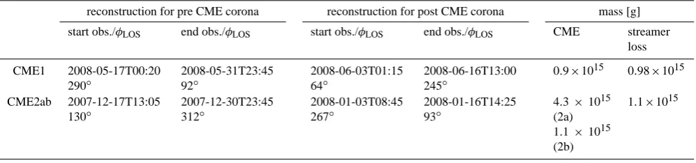
Table 1. Observation periods of input images for the tomographic reconstructions, and masses of the CMEs and streamer belt losses in the CME impacted regions (areas bounded by white square and round lines in Figs. 1, 3, 5, 7; also see Sect. 3 of the text).

reconstruction for pre CME corona reconstruction for post CME corona mass [g]

start obs./φLOS end obs./φLOS start obs./φLOS end obs./φLOS CME streamer loss

CME1 2008-05-17T00:20 290◦

2008-05-31T23:45 92◦

2008-06-03T01:15 64◦

2008-06-16T13:00 245◦

0.9×1015 0.98×1015

CME2ab 2007-12-17T13:05 130◦

2007-12-30T23:45 312◦

2008-01-03T08:45 267◦

2008-01-16T14:25 93◦

4.3× 1015 (2a) 1.1× 1015 (2b)

1.1×1015

the number of iterations, and value of µ. The value of µ

was chosen using the cross-validation method (Frazin and Janzen, 2002). The iterations are performed until the first term in Eq. (1) becomes slightly less than the data noise level which is essentially the Poisson noise in the data.

In order to increase the contribution of signals from those LOS which pass through the low density regions, and to re-duce the artifacts in the numerical reconstruction at larger distances from the Sun, a weighting function (or precondi-tioning) was applied. The regularization parameter and num-ber of iterations were chosen by cross-validation method. Detailed describtion of the used tomography method can be found in Kramar et al. (2009). As an output from the in-version we have 3-D electron density reconstruction of the corona at heliospheric distances from 1.5 to 4.0R.

Preliminary error analysis shows that the error due to sparseness of the data (2–3 per day) and regularization is of order 10 %, and the error due to non-stationarity of the corona during the period of observations (typically 14 days) could be up to 50 %. More detailed analysis of the error for the method is to be presented in the forthcoming paper.

3 Pre- and post-CME coronal streamer belt structure We analized pre- and post-CME coronal streamer belt struc-ture for two CME cases:

1. slow CME on 1 June 2008 (CME1).

2. two fast CMEs on 31 December 2007 (CME2a) and 2 January 2008 (CME2b).

The source regions of these two fast CMEs are very close to each other and located in the same active region near the Sun’s surface. Taking also into account that these CMEs oc-cured within a time interval of two days, we join them in one case study.

To reconstruct the 3-D electron density for pre- and post-CME corona, we used STEREO-B/COR1 data collected dur-ing a half of the solar rotation period just before and after

a CME. The starting and ending observation dates and cor-responded Carrington longitudes of STEREO-B spacecraft,

φLOS, are summarized in Table 1. Note, that the longitude decreases during the observations.

3.1 CME on 1 June 2008 (CME1)

The CME1 is a slow CME. The two most characteristic fea-tures found for this CME are (Robbrecht et al., 2009): (i) it contains a significant mass, and (ii) it was not found clear on-disk signatures to be identified as a source region for this CME (Robbrecht et al., 2009).

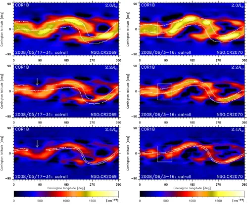
As the CME1 happened on 1 June 2008, to reconstruct the 3-D electron density in the corona before and after the CME, we used STEREO-B/COR1 data collected during a half of the solar rotation period just before and after the CME, i.e. during 17–31 May 2008 for the pre-CME density reconstruc-tion, and during 3–16 June 2008 for the post-CME density reconstruction (see Table 1). The spherical cross-sections of the reconstructed electron densities at heliocentric distances 2.0, 2.2 and 2.4Rare presented in Fig. 1. The independent localizations of the CME (Robbrecht et al., 2009) by several methods, indicates that the density decreases significantly in the streamer belt near Carrington longitude of 80◦is caused by the CME.

This region was in plane of the sky (POS) position for STEREO-B spacecraft on 26 May at 01:50 UT (east limb) and 8 June at 15:12 UT (west limb). So, the pre- and post-CME density reconstructions of the post-CME1 coronal region at 80◦ longitude reflects state of the corona at times about 4–5 days before and 7–8 days after the CME (STEREO-B for shifts for about 13.3◦ in longitude per day during the observational period). So, as seen from Figs. 1 and 2, the post-CME density remains significantly reduced in compar-ison with pre-CME state for at least about 7–8 days in the CME region.

1022 M. Kramar et al.: On the influence of CME on the 3-D coronal electron density

M. Kramar: On the influence of CME on the 3D coronal electron density 7

Fig. 1. Spherical cross-section of the reconstructed electron density in square root scale at heliocentric distances2_.0_,2_.2_and2_.4_R⊙(the

distances are shown in the right upper corners). The reconstruction for the period before the CME of June 1st, 2008 is shown on the left panel while the reconstruction for the period after this CME is shown on the right panel. The white lines are the boundaries between closed and open magnetic field lines for PFSS model with source surface at2_.5_{R⊙corresponded for CR 2069 and CR 2070, i.e. periods approximately}

before and after the CME. The part of the lines on the left panel between Carrington longitudes50_and110◦

are not shown in order to more clearly show the connecting structure in this region (marked with arrow). However the lines in this region are almost horizontal.

Fig. 1. Spherical cross-section of the reconstructed electron density in square root scale at heliocentric distances 2.0, 2.2 and 2.4R(the distances are shown in the right upper corners). The reconstruction for the period before the CME of 1 June 2008 is shown on the left panel while the reconstruction for the period after this CME is shown on the right panel. The white lines are the boundaries between closed and open magnetic field lines for PFSS model with source surface at 2.5Rcorresponded for CR 2069 and CR 2070, i.e. periods approximately before and after the CME. The part of the lines on the left panel between Carrington longitudes 50 and 110◦are not shown in order to more clearly show the connecting structure in this region (marked with arrow). However the lines in this region are almost horizontal.

110◦, latidudes from−30 to 25◦, and heliocentric distance from 1.5 to 3.6R. As the reconstructions gives the elec-tron density in physical units, we can calculate the mass lost by the corona within this region. So, assuming 10 % helium abundance which corresponds to mass per electron number equal to 1.974×10−24g (routine ne2mass in SolarSoft IDL library), we found the mass lost is 9.8×1014g. The mass of the CME measured in COR1 FOV is∼8×1014g (see ap-pendix for description). The maximal mass of the CME mea-sured in COR1 FOV estimated by Robbrecht et al. (2009) has about the same value of∼9×1014g. This fact is evidence

that material the CME consists of could be originated mainly from the streamer belt. However, it is difficult to make a final conclusion about the origin of the CME’s material be-cause our estimation of the mass loss of the streamer is based on the reconstructions of the corona from 1.5R. So, we do not know the pre- and post CME density below 1.5R.

M. Kramar et al.: On the influence of CME on the 3-D coronal electron density 1023

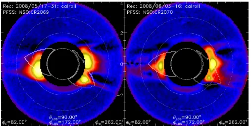
Fig. 2. Cross-sections of the reconstructed electron density in square root scale by a plane perpendicular to a LOS with Carrington longitude of 172◦and colatidude of 90◦. The reconstruction for the period before a CME of 1 June 2008 is shown on the left side while the reconstruc-tion for the period after this CME is shown on the right side. The white contour lines are the boundaries between closed and open magnetic field lines for a PFSS model with source surface at 2.5Rfor CR 2069 and CR 2070, i.e. periods approximately before and after the CME. The white circles mark heliospheric distances for 1, 2 and 3R.

8 M. Kramar: On the influence of CME on the 3D coronal electron density

Fig. 2. Cross-sections of the reconstructed electron density in square root scale by a plane perpendicular to a LOS with Carrington longitude of172◦

and colatidude of 90◦

. The reconstruction for the period before a CME of June 1st, 2008 is shown on the left side while the reconstruction for the period after this CME is shown on the right side. The white contour lines are the boundaries between closed and open magnetic field lines for a PFSS model with source surface at2_.5_{R⊙for CR 2069 and CR 2070, i.e. periods approximately before and after}

the CME. The white circles mark heliospheric distances for1_,2_and3_R⊙.

Fig. 3. Difference in reconstructed electron density for the periods after the CME of June 1st, 2008 (CME1) and before. The spherical cross-sections are shown at heliocentric distances2_.0_and2_.4_{R⊙(the distances are shown in the right upper corners).}

Fig. 3. Difference in reconstructed electron density for the periods after the CME of 1 June 2008 (CME1) and before. The spherical cross-sections are shown at heliocentric distances 2.0 and 2.4R(the distances are shown in the right upper corners).

streamer belt could be partially filled by the plasma. There-fore our estimation of mass lost by the streamer belt could be a lower limit.

The white contour lines in Fig. 1 represent the boundaries between closed and open magnetic field lines in potential field source surface model (PFSS) with the source surface lo-cated at 2.5Rfor the Carrington rotations (CR) correspond to p and post-CME times, i.e. CR 2069 and CR 2070,

1024 M. Kramar et al.: On the influence of CME on the 3-D coronal electron density

M. Kramar: On the influence of CME on the 3D coronal electron density 9

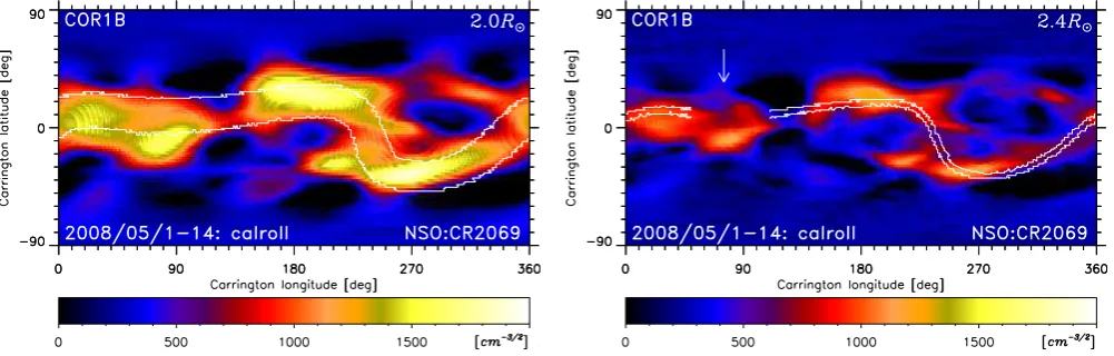
Fig. 4. Spherical cross-section of the reconstructed electron density in square root scale at heliocentric distances2_.0_and2_.4_{R⊙(the distances}

are shown in the right upper corners). The reconstruction based on data obtained during May 1-14, 2008. The white lines are the boundaries between closed and open magnetic field lines for PFSS model with source surface at2_.5_{R⊙corresponded for CR 2069. The part of the}

lines on the right panel between Carrington longitudes50_and110◦

are not shown in order to more clearly show the density structure in this region. However the lines in this region are almost horizontal.

Fig. 4. Spherical cross-section of the reconstructed electron density in square root scale at heliocentric distances 2.0 and 2.4R(the distances are shown in the right upper corners). The reconstruction based on data obtained during 1–14 May 2008. The white lines are the boundaries between closed and open magnetic field lines for PFSS model with source surface at 2.5Rcorresponded for CR 2069. The part of the lines on the right panel between Carrington longitudes 50 and 110◦are not shown in order to more clearly show the density structure in this region. However the lines in this region are almost horizontal.

The PFSS reconstructions are based on the magnetograph observations from the Earth. The NSO/GONG observations for CR 2069 ended on 2008-05-20T23:54 when Earth was at 262◦longitude, and for CR 2070 on 2008-06-16T23:54 when Earth was at 265◦ longitude. The Earth was at 80◦ longi-tude (CME1 region) on 2008-05-07T12:40 corresponding to CR 2069 and 2008-06-03T17:47 corresponding to CR 2070. On 2008-06-03T17:47, just after the CME1, the Earth was at 80◦_{longitude (CME1 region). This date corresponds to} CR 2070. Therefore we compare PFSS model for CR 2070 with the post-CME reconstruction. And this comparison has sence for longitudes around the CME1 region, but could be not valid for the rest of the corona because of the difference in the observation dates for data needed for the PFSS model and tomographic reconstruction.

The magnetograph data for the pre-CME1 period is ob-tained during about 2008-05-07T12:40 date corresponding to CR 2069. But presented on Figs. 1 and 2 the density recon-struction for the pre-CME1 period is based on data obtained during 17–31 May 2008, which is more than a week after the central meridian passage through CME1 region. Therefore it is useful to make another reconstruction for period of 1–14 May 2008 in order to look how the corona changes. Figure 4 shows the spherical cross-sections of the reconstructed elec-tron densities at heliocentric distances 2.0 and 2.4Rwhen input COR1B images for the inversion are from 1–14 May 2008. We can see similar density structure near Carrington longitude of 80◦as for the 17–31 May reconstruction.

Figure 2 represents cross-sections of the reconstructed electron density by a plane perpendicular to a LOS with Car-rington longitude of 172◦and latidude of 0◦. The reconstruc-tion for the period before a CME of 1 June 2008 is shown on the left side while the reconstruction for the period after this

M. Kramar et al.: On the influence of CME on the 3-D coronal electron density 1025

10 M. Kramar: On the influence of CME on the 3D coronal electron density

Fig. 5. Spherical cross-section of reconstructed electron density in square root scale at heliocentric distances 2_.0_, 2_.2_and2_.4_{R⊙ (the}

distances are shown in the right upper corners). The reconstruction for the period before CMEs of December 31st, 2007 and January 2nd, 2008 is shown on the left panel while the reconstruction for the period after these CMEs is shown on the right panel. The white lines are the boundaries between closed and open magnetic field lines for a PFSS model with source surface at2.5R⊙for CR 2064 and CR 2065, i.e.

periods approximately before and after the CMEs. Two rombs indicate the source regions for CME2ab. Circles shows the region used for the computation of the mass loss.

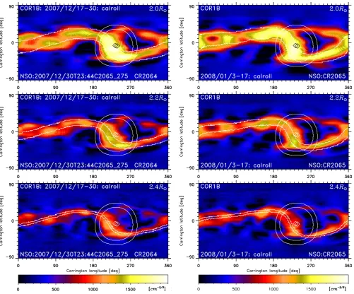
Fig. 5. Spherical cross-section of reconstructed electron density in square root scale at heliocentric distances 2.0, 2.2 and 2.4R(the distances are shown in the right upper corners). The reconstruction for the period before CMEs of 31 December 2007 and 2 January 2008 is shown on the left panel while the reconstruction for the period after these CMEs is shown on the right panel. The white lines are the boundaries between closed and open magnetic field lines for a PFSS model with source surface at 2.5Rfor CR 2064 and CR 2065, i.e. periods approximately before and after the CMEs. Two rombs indicate the source regions for CME2ab. Circles shows the region used for the computation of the mass loss.

Carrington longitude reflects state of the corona at times about a day before and 7–12 days after the CMEs (STEREO-B shifts for about 13.2◦in longitude per day during the ob-servational period).

The NSO/GONG observations for CR 2064 PFSS model ended on 5 January 2008 23:34 UT when Earth was at 256◦ longitude, and for CR 2065 on 1 February 2008 23:44 UT when Earth was at 260◦ longitude. The Earth was at 235◦ longitude (CME2ab region) on 11 December 2007 05:05 UT corresponding to CR 2064 and 7 January 2008 13:00 UT cor-responding to CR 2065.

As integral NSO/GONG harmonic coefficients for CR 2064 at about 235◦longitude are based on observations both before and after CME2ab date, for the PFSS model for the pre-CME period we used the harmonic coefficients based on observations finished on 30 December 2007 23:44 UT when Earth was at 334◦_longitude.

1026 M. Kramar et al.: On the influence of CME on the 3-D coronal electron density

Fig. 6. Cross-sections of the reconstructed electron density in square root scale by a plane perpendicular to a LOS with Carrington longitude of 325◦and colatidude of 90◦. The reconstruction for the period before the CME2ab is shown on the left side while the reconstruction for the period after CME2ab is shown on the right side. The white contour lines are the boundaries between closed and open magnetic field lines for a PFSS model with source surface at 2.5Rfor CR 2064 and CR 2065, i.e. periods approximately before and after the CME. The white circles mark heliospheric distances for 1, 2 and 3R.

M. Kramar: On the influence of CME on the 3D coronal electron density 11

Fig. 6. Cross-sections of the reconstructed electron density in square root scale by a plane perpendicular to a LOS with Carrington longitude of325◦_{and colatidude of}90◦_{. The reconstruction for the period before the CME2ab is shown on the left side while the reconstruction for}

the period after CME2ab is shown on the right side. The white contour lines are the boundaries between closed and open magnetic field lines for a PFSS model with source surface at2.5R⊙for CR 2064 and CR 2065, i.e. periods approximately before and after the CME. The white

circles mark heliospheric distances for1_,2_and3_R⊙.

Fig. 7. Difference in reconstructed electron density for the periods after and before the CMEs of December 31, 2007 (CME2a) and January 2, 2008 (CME2b). The spherical cross-sections are shown at heliocentric distances2_.0_and2_.4_{R⊙(the distances are shown in the right upper}

corners).

Fig. 7. Difference in reconstructed electron density for the periods after and before the CMEs of 31 December 2007 (CME2a) and 2 January 2008 (CME2b). The spherical cross-sections are shown at heliocentric distances 2.0 and 2.4R(the distances are shown in the right upper corners).

circle line in Figs. 5 and 7) We can estimate the mass lost by the corona in the region within this cone and heliocen-tric distances from 1.5 to 3.6R. Assuming 10 % of helium abundance, which corresponds to mass per electron number equal to 1.974×10−24g (routine ne2mass in SolarSoft IDL library), we found a mass loss of 1.1×1015g. Note, that this number is a mass difference within the selected region, i.e.

it takes into account also increase of the mass for whatever reason caused by the CMEs or not . The only negative part of the difference gives a number of 2.5×1015g.

M. Kramar et al.: On the influence of CME on the 3-D coronal electron density 1027 streamer belt mass loss for CME2ab case is less than total

masses of CME2ab. Moreover, the PFSS model for the pe-riod before CME2ab is in much better agreement with the re-constructed electron density structure than the PFSS model for the period before CME1. So, these properties could be explained that CME2ab has source region deep in the corona near the photosphere which is clearly seen in EUVI 304 and during their expansion the CME2ab “pushed out” surround-ing materia. However, the lower number of mass loss could also be explained by the fact that the CME2ab originates in an active region with higher density and after the CMEs the density above this active region was “recovered” faster than time needed to collect data for tomographic reconstruction.

Figure 6 represents cross-sections of the reconstructed electron density by a plane perpendicular to a LOS with Car-rington longitude of 325◦and latidude of 0◦. The reconstruc-tion for the period before CME2ab is shown on the left side while the reconstruction for the period after these CMEs is shown on right side. The east sides from the Sun corre-spond to the region with Carrington longitude of 235◦, i.e. where the CME2ab took place. We see that the height of the streamer in the CME region after the CMEs is relatively slightly reduced in contrary with the CME1 case.

4 Conclusions

1. To our knowledge this is the first direct evidence (elim-inated from the LOS effect) of the streamer blow out effect caused by the slow CME. Llebaria et al. (2006) made a statistical analysis of the interaction of CMEs with the streamer belt and have found that 72 % cases of slow CMEs caused dimming in the streamer (i.e. steep decrease of the streamer brightness after the event) while this effect occured only for 18 % of the investi-gated fast CMEs.

The height of the streamer in the CME region after the CME1 is significantly reduced in contrast to with the CME2ab case where this height remains almost the same as before as well after the CME2ab.

2. The potential magnetic field configuration in CME1 ini-tiation region before the CME occured does not agree with the coronal density structure, while after the CME the agreement between the field and density is much better. This could be a manifistation of that the field before the CME1 is non-potential and after the CME1 the field relaxes towards a more potential state. Also, the interpretation of the position of heliospheric current sheet based on PFSS model during a pre-CME period could be very questionable.

On the other hand, for the fast CME2ab the PFSS model and the reconstructed streamer belt structure above the source region are in good agreement both before and after the

CME2ab occurred. On smaller scales inside the active region the PFSS model could not be validated. This could be indi-cation of different initiation and/or propagation mechanisms for these two cases. Particularly, the source region for CME1 could be located higher in the corona than for CME2ab.

The present paper is a first step in the analysis of inter-actions of CMEs with the streamer belt structure using 3-D structure of the belt obtained from the tomographic struction. We considered here only two cases. A 3-D recon-struction of the type discussed in this paper could be pro-duced for almost every Carrington rotation during STEREO operational period in a robust way allowing a more system-atic study.

Appendix A

CME mass calculation

We estimated the masses of CME2a and CME2b in the fol-lowing way:

m=X i

B_obs(xi,yi)

Be(xi,yi,ψ )

·1.97×10−24g, (A1)

where the ratio of B_obs(xi,yi)/Be(xi,yi,ψ ) is the excess

number of electrons, B_obs(xi,yi)is the excess brightness

observed in a given pixel with index number i at loca-tion (xi,yi)in the plane of the sky (POS),Be(xi,yi,ψ ) is

the brightness of a single electron at that location at an-gle ψ away from POS derived from the Thompson scat-tering equations (Billings, 1966). The angle ψ at loca-tion (x0,y0) can be computed by the following equations:

ψ=atan(z0/ q

x₀2+y₀2). The error in CME’s mass estima-tion could be up to 50 % (Vourlidas et al., 2000).

Acknowledgements. Thanks to Bernd Inhester for useful disscus-sions and comments that help to improve the paper. Also thanks to Gordon Petrie for usefull comments about potential field re-construction methods. Thank to unknown referee for useful com-ments helped to improve the paper. This research was partially supported by NSF National Space Weather Program grant num-ber AGS0819971.

Topical Editor R. Forsyth thanks F. Auchere and another anony-mous referee for their help in evaluating this paper.

References

Altschuler, M. D. and Newkirk, G.: Magnetic Fields and the Struc-ture of the Solar Corona. I: Methods of Calculating Coronal Fields, Solar Phys., 9, 131–149, 1969.

Billings, D. E.: A Guide to the Solar Corona, New York: Academic Press, 1966.

1028 M. Kramar et al.: On the influence of CME on the 3-D coronal electron density

Demoulin, P., Cuperman, S., and Semel, M.: Determination of force-free magnetic fields above the photosphere using three-component boundary conditions. II – Analysis and minimization of scale-related growing modes and of computational induced singularities, Astron. & Astrophys., 263, 351–360, 1992. Forbes, T. G.: A review on the genesis of coronal mass ejections, J.

Geophys. Res., 105, 23153–23166, 2000.

Frazin, R. A. and Janzen, P.: Tomography of the Solar Corona. II. Robust, Regularized, Positive Estimation of the Three-dimensional Electron Density Distribution from LASCO-C2 Po-larized White-Light Images, Astrophys. J., 570, 408–422, 2002. Frazin, R. A. and Kamalabadi, F.: Rotational Tomography For 3d Reconstruction Of The White-Light And Euv Corona In The Post-Soho Era, Solar Phys., 228, 219–237, 2005.

Hudson, H. S., Bougeret, J.-L., and Burkepile, J.: Coronal mass ejections: overview of observations, Space Sci. Rev., 123, 13– 30, 2006.

Jiao, L., McClymont, A. N., and Miki´c, Z.: Reconstruction of the Three-Dimensional Coronal Magnetic Field, Solar Phys., 174, 311–327, 1997.

Judge, P. G.: Spectral Lines for Polarization Measurements of the Coronal Magnetic Field. V. Information Content of Magnetic Dipole Lines, Astrophys. J., 662, 677–690, 2007.

Klimchuk, J. A.: Theory of Coronal Mass Ejections, in: Space Weather (Geophysical Monograph 125), edited by: Song, P., Singer, H., and Siscoe, G., American Geophysical Union, 143, 2001.

Kramar, M. and Inhester, B.: Inversion of coronal Zeeman and Hanle observations to reconstruct the coronal magnetic field, Memorie della Societa Astronomica Italiana, 78, 120–125, 2007. Kramar, M., Inhester, B., and Solanki, S. K.: Vector tomography for the coronal magnetic field. I: longitudinal Zeeman effect mea-surements, Astron. Astrophys., 456, 665–673, 2006.

Kramar, M., Jones, S., Davila, J., Inhester, B., and Mierla, M.: On the Tomographic Reconstruction of the 3D Electron Density for the Solar Corona from STEREO COR1 Data, Solar Phys., 259, 109–121, 2009.

Lin, H., Kuhn, J. R., and Coulter, R.: Coronal Magnetic Field Mea-surements, Astrophys. J., 613, 177–180, 2004.

Llebaria, A., Saez, F., Lamy, P., Robelus, S., and Boursier, Y.: Inter-actions of CMEs with the streamer belt, ESASP, 617, 135–138, 2006.

Mikic, Z. and Lee, M. A.: An introduction to theory and models of CMEs, shocks, and solar energetics particles, Space Sci. Rev., 123, 57–80, 2006.

Quemerais, E. and Lamy, P.: Two-dimensional electron density in the solar corona from inversion of white light images – Appli-cation to SOHO/LASCO-C2 observations, Astron. Astrophys., 393, 295–304, 2002.

Robbrecht, E., Patsourakos, S., and Vourlidas, A.: No Trace Left Behind: Stereo Observation of a Coronal Mass Ejection without Low Coronal Signatures, Astrophys. J., 701, 283–291, 2009. Sakurai, T.: Computational modeling of magnetic fields in solar

active regions, Space Sci. Rev., 51, 11–48, 1989.

Thompson, W. T. and Reginald, N. L.: The Radiometric and Point-ing Calibration of SECCHI COR1 on STEREO, Solar Phys., 250, 443–454, 2008.

Tikhonov, A. N.: Solution of incorrectly formulated problems and the regularization method, Soviet Math. Dokl., 4, 1035–1038, 1963.

Tomczyk, S., Card, G. L., Darnell, T., Elmore, D. F., Lull, R., Nel-son, P. G., Streander, K. V., Burkepile, J., Casini, R., and Judge, P. G.: An Instrument to Measure Coronal Emission Line Polar-ization, Solar Phys., 247, 411–428, 2008.

Van de Hulst, H. C.: The electron density of the solar corona, Bull. Astron. Inst. Netherlands, 11, 135–150, 1950.

Vourlidas, A., Subramanian, P., Dere, K. P., and Howard, R. A.: Large-angle spectrometric coronagraph measurements of the en-ergetics of coronal mass ejections, Astrophys. J., 534, 456–467, 2000.

Wiegelmann, T.: Nonlinear force-free modeling of the so-lar coronal magnetic field, J. Geophys. Res., 113, A03S02, doi:10.1029/2007JA012432, 2008.

Wiegelmann, T., Lagg, A., Solanki, S. K., Inhester, B., and Woch, J.: Comparing magnetic field extrapolations with measurements of magnetic loops, Astron. Astrophys., 433, 701–705, 2005. Zidowitz, S.: Coronal structure of the Whole Sun Month: A