Solving the singular two-dimensional fourth order problem by the mortar spectral element method

R E S E A R C H

Open Access

Solving the singular two-dimensional

fourth order problem by the mortar spectral

element method

Mohamed Abdelwahed, Azhar Al Salam and Nejmeddine Chorfi

*_{Correspondence:}

nejmeddine.chorfi@yahoo.com Department of Mathematics, College of Sciences, King Saud University, Riyadh, Saudi Arabia

Abstract

In this work, we implement the mortar spectral element method for the biharmonic problem with a homogeneous boundary condition. We consider a polygonal domain with corners which relies on the mortar decomposition domain technique. We propose the Strang and Fix algorithm, which permits to enlarge the discrete space of the solution by the first singular function. The interest of this algorithm is the approximation of the solution and the leading singular coefficient which has a physical significance in the propagation of cracks. We give some numerical results which confirm the optimality of the order of the error.

Keywords: Biharmonic equation; Fourth order problem; Singularity; Strang and Fix algorithm; Mortar spectral element method

1 Introduction

Consider the fourth order problem with homogeneous boundary conditions called the biharmonic homogeneous problem

⎧ ⎪ ⎪ ⎨ ⎪ ⎪ ⎩

2ϕ=f in,

ϕ= 0 on∂,

∂ϕ

∂n= 0 on∂,

(1)

whereis a polygonal domain ofRd_{,d= 2, 3 and∂is a Lipschitz-continuous boundary}

of[1].

This type of problem is involved in many problems in the mechanics of a continuous medium for both fluids and solids. Other applications such as some models in control theory involve fourth order operators. The solutionϕof this type of problem is composed of regular and singular parts [2–4]. To weaken the effect of the geometric singularity, we apply the method of domain decomposition without overlapping. This method is associ-ated with the mortar method [5] with variational spectral elements discretization. Since the discrete solution (polynomial) is regular on each sub-domain of the decomposition, then the non-conformity results in the imposition of an integral matching condition on the solution and its normal derivative. This matching condition type is weak. It allows great

geometric flexibility and is perfectly suited to parallel computing. The approximation of a singular part of the solution using the finite element method is presented in [6, 7]. In [8], the authors prove an optimal approximation by polynomials using the spectral method. In this work we will use these results to implement the mortar spectral elements method for the Strang and Fix algorithm [9] in the case of the biharmonic problem. It consists in enlarging the discrete space by the first singular function. The polynomial basis of the new discrete space permits us to approximate the solution and the leading singularity coeffi-cient. This coefficient has a physical signification in the crack propagation [10–13]. We begin by writing the matrix system, then we use the conjugate gradient algorithm to solve it. We illustrate the good convergence of the presented method through numerical error curves. This work is an extension of the work presented in [14] for the case of domain with geometric singularity.

An outline of this paper is as follows. In Sect. 2, we present the geometry of the do-main and a continuous problem, we give singular functions and some regularity results. In Sect. 3, we present a discrete problem. The error result obtained from the discretization of the biharmonic problem by the mortar spectral method is showed in Sect. 4. Section 5 is devoted to the implementation of the mortar spectral element method. We describe the matrix system and its resolution algorithm. Finally, we present some numerical results which confirm the interest in the method.

2 Continuous problem

We decompose the domainintoKrectanglesk, 1≤k≤K, such that

=

K

k=1

k and k∪l=∅, 1≤k=l≤K.

We designate byk,j, 1≤j≤4, the sides of the sub-domaink, 1≤k≤K, and

γ_kl=k∩l, 1≤k=l≤K

the interface of the decomposition.

The skeleton of the decomposition is defined as follows:

S=

K

k=1 4

j=1 k,j.

We denote byVthe set of vertices of the sub-domain for our decomposition. Letk(m),j(m) be an open set of segments disjoint two by two for an integermin a setM. Then

S=

m∈M

k(m),j(m).

We called mortars the segmentsk(m),j(m)_{,m∈M. The intersection of a sub-domain}

k,

1≤k≤K, with the boundary∂is reduced to an element ofV.

2π. Since the treatment of singularities is local, we reduce our study to a single geometric vertex v andωthe associated angle. We suppose that the sides of sub-domains are parallel to the scale axis of origin v. We consider (r,θ) the polar coordinates withrthe distance from a point to the vertex v and the lineθ= 0 contains a side of∂.

We need the following conformity hypothesis for our analysis later.

Assumption 1 Letbe the union of sub-domains which contain the vertex v. We sup-pose that the decomposition of the domainis geometric conforming (fork andl

included in,¯k∩ ¯l=kl,k=l,klis an edge of bothkandl).

Problem (1) is equivalent to the following variational formulation: Forf ∈H–2_{(), findϕ∈H}2

0() for allψ∈H02()

a(ϕ,ψ) =f,ψ , (2)

where a(ϕ,ψ) =ϕ:ψdx dyand·,· is the duality product betweenH–2_{() and}

H2 0().

According to the Lax–Milgram theorem, problem (2) has a unique solution, since the bilinear forma(·,·) is continuous inH2

0()×H02() and coercive inH02(). We consider the following stability condition:

ϕ_H2₍₎≤Cf_H–2₍₎,

whereCis a positive constant which is dependent just on[15, 16].

For handling the singularities, we consider the bi-Laplacian characteristic equation

sin(ωz)2=z2sinω2 (3)

[2, 3] and

η(ω) =infReal(z),zis solution of (3),z=±1.

The solution of problem (1) is decomposed into the formϕ=ϕR+λS1 such thatϕR∈ Hs+2_{(),s< 1 +η(ω) and}

ϕRHs+2₍₎+|λ₁| ≤Cf_Hs–2₍₎,

whereCis a positive constant,λ1is the first singular coefficient and

S1(r,θ) =r1+η(ω)φ(θ). (4)

•Ifω=3₂π, we haveη(ω) = 0.54484,s< 1.544, andφ(θ) = 2.093(cos(0.459θ)–cos(1.544θ))+ 1.093(2.193sin(0.459θ) –sin(1.544θ)).

However, iff ∈Hs–2_{() withs< 2.908, we can still push the decomposition of the} solu-tion of problem (1) as

The regular part of the solutionϕ˜Ris in the spaceHs+2() such that

˜ϕRHs+2₍₎+|λ₁|+|λ₂| ≤Cf_Hs–2₍₎,

whereCis a positive constant andλ2is the second singular coefficient. The second sin-gularity function is defined as

S2(r,θ) =r1+η1(ω)ς(θ), (6)

whereη1(ω) is the second real solution of equation (3) in the band 0 < Real(z) < 1(η1(3₂π) 0.908529) and ς(θ) = 4.302(cos(0.092θ) – cos(1.908θ)) – 1.815(10.869sin(0.092θ) – 0.524sin(1.908θ)).

•Ifω= 2π, we haveη(ω) = 0.5,s< 1.5, and

S1(r,θ) =r32

sin3

2θ– 3sin θ 2

+

cos3

2θ–cos θ 2

,

S2(r,θ) =r52

sin5

2θ– 5sin θ 2

+

cos5

2θ–cos θ 2

.

Sincef belongs toHs–2(), thenϕ˜Rbelongs toHs+2() fors< 2, 5 such that

˜ϕRHs+2₍₎+|λ1|+|λ2| ≤Cf_Hs–2₍₎,

whereCis a positive constant.

3 Discrete problem

We introduce the discretization parameterδ= (Nk)1≤k≤K, wherePNk(k), 1≤k≤K, are the approximation polynomials with degrees less or equal toNkin each sub-domaink.

We define the mortars functions space

Wδ=

(0,1)∈PNk(m)(k(m))×PNk(m)(k(m));0/γm=ψδ/k(m),j(m)

and1/γm=

∂ψδ

∂n

k(m),j(m)∀m∈M

,

whereψδis a test function.

The Galerkin method with numerical integration is used for spatial discretization. To take into account boundary conditions of the fourth order studied problem, we choose a quadrature formula presented in the following lemma.

Lemma 3.1 There existξj, 1≤j≤N– 1 (N≥2),a set of unique pointsρj, 1≤j≤N– 1, a set of unique positive realsρ+,ρ–such that∀∈P2N–1(]–1, 1[)

1

–1

(x)dx=

N–1

j=1

(ξj)ρj+(–1)ρ–+(1)ρ+. (7)

Proof See [17] for the calculation ofρj,ξj; 1≤j≤N– 1 (the zeros of the derivative of the

Definition 3.2 Forϕ,ψ two continuous functions on¯ˆ = [–1, 1]×[–1, 1] such thatϕ= ψ= 0 on∂, we define

•

(ϕ,ψ)N= N–1

i=1

N–1

j=1

ϕ(ξi,ξj)ψ(ξi,ξj)ρiρj

the discrete scalar product. •

(ϕ,ψ)Nk=

|k|

4

Nk–1

i=1

Nk–1

j=1

ϕ◦Bk (ξi,ξj)

ψ◦Bk (ξi,ξj)ρiρj,

whereBkis the bijection fromˆ tok.

• Xδis the space of functionsψδsuch that

– ψ_δk=ψδ/k∈PNk(k),1≤k≤K, – ψδ=∂ψ_∂nδ = 0on∂,

– there exist(0,1)∈Wδ/∀1≤k≤K,1≤j≤4,

k,j(ψδ–0)(τ)μ(τ)dτ= 0and

k,j( ∂ψδ

∂n –1)(τ)μ(τ)dτ= 0∀μ∈PNk–4( k,j_).

The discrete problem of continuous problem (1) is as follows. Forf ∈C(), findϕδ∈Xδ such that

∀ψδ∈Xδ, aδ(ϕδ,ψδ) = (f,ψ)δ,

whereaδ(ϕδ,ψδ) =

K

k=1(ϕδk,ψδk)Nk and (f,ψδ)δ= K

k=1(f,ψδk)Nk. We proceed now to the enlargement of the discrete spaceXδto the space

X_δ∗=Xδ+RS1,

using the Strang and Fix algorithm [9], whereS1is the first singular function. We obtain then forϕ_δ∗=ϕδ+αS1andψδ∗=ψδ+βS1inXδ∗

a∗δ

ϕδ∗,ψδ∗ = K

k=1

ϕδk,ψδk _Nk+α

k

ψδkS1dx+β

k

ϕkδS1dx

+αβ

k

(S1)2dx

.

We refer to the appendix of [10] for the algorithm which permits to compute the singular integral

kψ k δS1dx.

We consider the following discrete problem: Findϕ∗_δ∈Xδ∗such that

∀ψ_δ∗∈Xδ∗, a∗δ

ϕ_δ∗,ψ_δ∗ =

K

k=1

k

fψ_δ∗_kdx, (8)

We define two norms on the spaceXδ∗

ϕ_δ∗_∗1=

K

k=1

ϕk_δ2_H2₍ k)+|α|

2_S 1/k

2

H2₍ k)

1/2

and

ϕ_δ∗_∗2= _K

k=1

ϕ_δ∗2_H2₍ k)

1/2 .

Proposition 3.3 For f ∈L2(),the discrete problem(8)has a unique solutionϕ_δ∗ in Xδ∗

and

ϕ∗

δ_∗2≤CfL2₍₎.

Proof To study problem (8), we begin by giving the properties of the bilinear forma∗δ(·,·)

(see [18], Prop. 5.2, for the proof ).

There exist two positive functionsC1andC2independent ofδsuch that for allϕ∗δ,ψδ∗

inX∗δ

a∗δ

ϕ_δ∗,ψ_δ∗ ≤C1ϕδ∗_∗1ψδ∗_∗1 (9)

and

a∗δ

ϕ_δ∗,ψ_δ∗ ≥C2ϕδ∗

2

∗2. (10)

Using the fact that · ∗1 and · ∗2are equivalent with a constant depending on the parameter δ ([18] Prop 5.1), an inf-sup condition will be showed for the bilinear form

a∗δ(·,·) using the norm∗1(see [18], Prop. 5.5, for the proof ).

4 Error estimate

Proposition 4.1 Let f in Hs–2_{()for s> 0,then,for all> 0,}

ϕ–ϕ_δ∗

L2₍₎≤C

N–2

_K

k=1

N–σk k

fHs–2₍₎,

whereσk, 1≤k≤K,verifies

σk=

⎧ ⎪ ⎪ ⎨ ⎪ ⎪ ⎩

s– 2 ifkdoes not contain any vertices of,

inf(s– 2, 2η1(π₂) –ε) ifkcontains one vertex ofother thanv,

inf(s– 2, 2η1(ω) –ε) ifkcontainsv,

(11)

and N=inf_1≤k≤KNk.

Proof By inf-sup condition on the bilinear forma∗δ(·,·), there exists a constantνsuch that

∀ψ_δ∗∈Xδ∗; sup t_δ∗∈X_δ∗

a∗δ(ψδ∗,tδ∗)

t_δ∗∗1 ≥ νψ∗

Using (12) and the Strang lemma, we obtain

ϕ–ϕδ∗∗1≤C

inf

ψ_δ∗∈X_δ∗

ϕ–ψ_δ∗_∗1+ sup

ω∗_δ∈X∗_δ

a(ψ_δ∗,ω∗_δ) –a∗_δ(ψ_δ∗,ω∗_δ)

ω∗_δ∗1

× sup

ω∗_δ∈X_δ∗

K k=1

K l=k+1(

γkl ∂(ϕ)

∂n [ω∗δ]dx–

γklϕ[ ∂ω∗_δ

∂n]dx) ω∗_δ∗1

(13)

nis the outside normal and [ω] is the jump ofωon the interfaces.

We will estimate the terms of inequality (13) to obtain the order of convergence. Using the fact that the singular functionS1is regular in the neighborhood of v, the jump terms (ω∗_δk–ω∗_δl) (respectively (∂ω∗δk

∂n – ∂ω∗_δl

∂n )) are reduced through each interfaceγklto (ωδk–ωδl)

(respectively (∂ωδk ∂n –

∂ωδl

∂n )). Furthermore, using the hypothesis of conformity on, these

obtained quantities vanish. Moreover,ϕ=ϕRon/; we obtain then

γ_kl

∂(ϕ)

∂n [ωδ]dx+

γ_kl ϕ ∂ωδ ∂n dx = γkl ∂(ϕR)

∂n (0–ωδk)dx+

γkl ∂(ϕR)

∂n (0–ωδl)dx

+

γ_kl

(ϕR)

1–

∂ωδk

∂n

dx+

γ_kl

(ϕR)

1–

∂ωδl

∂n

dx,

where0(respectively1) is the mortar function associated withωδ (respectively∂ω_∂nδ).

We then obtain the following [19]:

K

k=1

K

l=k+1

γkl ∂(ϕR)

∂n [ωδ]dx+

γkl ϕR ∂ωδ ∂n dx ≤c K k=1 4 j=1 inf

ψkj∈P_Nk–4(kj) ∂(ϕR)

∂n –μkj

(H3/2₍kj₎₎

+ inf

ψkj∈PNk–4(kj)

ϕR–μkj(H1/2₍kj₎₎

. (14)

We have by definition ofX∗_δ

inf

ψ_δ∗∈X∗_δ

ϕ–ψδ∗_∗1≤C inf vδ∈Xδ–

ϕR–ψδ∗1,

where

X_δ–=ψδ∈Xδ;ψδk∈PN–1(k)

.

Choosingψ_δ∗=ψδ∈Xδ–and by the exactness of the quadrature formula (7)

sup

ω∗_δ∈X∗_δ

a(ψδ∗,ω∗δ) –a∗δ(ψδ∗,ω∗δ)

Finally, by doing the sum of these results, we have

ϕ–ϕ_δ∗_∗1≤C

inf

ψδ∈X–δ

ϕ–ψδ∗1+

K

k=1 4

j=1

inf

ψkj∈P_Nk–4(kj) ∂ϕR

∂n –μkj

(H3/2₍kj₎₎

+ inf

μkj∈P_Nk–4(kj)

ϕR–μkj(H1/2₍kj₎₎

. (15)

Iff ∈Hs–2_{() forη(ω) <s<η(ω) + 2, thenϕ}

R∈Hs+2() and the trace (respectively the

nor-mal derivative trace) ofϕR∈Hs– 1

2(∂_k) (respectively∈Hs–23(∂_k)); 1≤k≤K. Choosing μkjandχkj, the orthogonal projections onPNk–4(kj), we deduce

ϕR–μkj(H1/2₍kj₎₎≤CN_k–sϕRHs+2₍ k)

and ∂ϕR

∂n –χkj

H–3/2₍kj₎≤

CN_k–sϕRHs+2₍ k).

Moreover, we obtain

inf

ψδ∈X–δ

ϕ–ψδ∗1≤C

K

k=1

N_k–sϕRHs+2₍ k).

Iff inHs–2_{(),s< 2 +η1(ω), whereη1(ω) is the second real solution of (3), in the band} 0 < Real(z) <s, then using (5) and Assumption 1, we show that

ϕ–ϕ_δ∗_∗1≤C

inf

ψδ∈X–δ

ϕR–ψδ∗1+ K

k=1 4

j=1

inf

μkj∈P_Nk–4(kj) ∂ϕ˜R

∂n –μkj

(H3/2₍kj₎₎

+ inf

χkj∈PNk–4(kj)

ϕ˜R–χkj(H1/2₍kj₎₎

.

We indicate that

inf

ψδ∈X–δ

ϕR–ψδ∗1≤C

inf

ψδ∈Xδ–

˜ϕR–ψδ∗1+|λ2| inf

ψδ∈Xδ–

S2–ψδ∗1

.

Using the results of the singular functions approximation through polynomials (see [8]), we obtain

inf

ψδ∈X–δ

S2–ψδ∗1≤CNε–2η1(ω) ∀ε> 0.

Then

inf

ψδ∈X–δ

ϕR–ψδ∗1≤CN2–s

therefore

ϕ–ϕ_δ∗_∗1≤CN2–sfHs–2₍₎ fors< 2 +η1(ω).

Using these results, we obtain, forf∈Hs–2_{(),s> 0, andε> 0,}

ϕ–ϕ_δ∗_∗1≤C

_K

k=1

N–σk k

fHs–2₍₎,

whereσkis given by (11).

By the Aubin–Nische duality, we obtain the desired estimation with theL2_norm.

Remark4.2 We denote that in the case of the crack (respectivelyω=3₂π) the convergence order isN–2_{(respectivelyN}–83_{). This demonstrates that the method is highly accurate.}

5 Numerical implementation and results

In this section we are interested in the implementation of the mortar method for the Strang and Fix algorithm in the case of a fourth order problem. The implementation is performed using the spectral elements method with a global algorithm for the resolution. In the spec-tral discretization the algorithmic aspect is mainly identical despite the diversity of the problems to be solved. The main ideas behind this algorithm are inspired by the works of Anagnostou [20] and Belhachmi and Bernardi [21].

The program is written in Matlab, which permits a good memory optimization and pro-vides a data structure depending on the initial geometry. The program has three modules corresponding to the three phases of the problem resolution. The first module is about the geometric aspect. The second module is related to the discretization of the problem which leads to the linear system. Finally, the last module is the resolution of the linear system and the exploitation of the results. This three components are programmed in a relatively general way and as much as possible are independent.

5.1 Choice of the basis

To describe algebraically the discrete problem (8), it is necessary to choose a basis of the space Xδ∗. This basis is defined naturally through local basis (on each sub-domain) and

therefore relative to the discretization.

For the quadrature formula, the number of equations is greater than the number of un-knowns. We neglect the firsti= 1 and the lasti=N– 1 in dimension 1. The basic polyno-mials for the Gauss–Lobatto quadrature formula are the Hermit interpolation polynomi-als that are defined on the interval ]–1, 1[ by

⎧ ⎨ ⎩

hi(ξj) =δij, 2≤j≤N– 2, 2≤i≤N– 2,

hi(–1) = 0, hi(1) = 0, hi(–1) = 0, hi(1) = 0, 2≤i≤N– 2.

⎧ ⎪ ⎪ ⎪ ⎪ ⎪ ⎨ ⎪ ⎪ ⎪ ⎪ ⎪ ⎩

h1(ξj) = 0, 2≤j≤N– 2,

h1(–1) = 1, h1(1) = 0, h₁(–1) = 1, h₁(1) = 0,

hN–1(ξj) = 0, 2≤j≤N– 2,

⎧ ⎪ ⎪ ⎪ ⎪ ⎪ ⎨ ⎪ ⎪ ⎪ ⎪ ⎪ ⎩

h0(ξj) = 0, 2≤j≤N– 2,

h0(–1) = 0, h0(1) = 0, h₀(–1) =h₀(1) = 0,

hN(ξj) = 0, 2≤j≤N– 2,

hN(–1) =hN(1) = 0, hN(–1) =hN(1) = 0.

We verify that these polynomials are represented by the formula

hi(x) =ci

(1 –x2₎2_L

N(x)

(x–ξ1)(x–ξi)(x–ξN–1)

, 2≤i≤N– 2,x∈]–1, 1[,

where the constantsciare given by

ci=

(ξi–ξ1)(ξi–ξN–1) N(N+ 1)(1 –ξi)2LN(ξi)

,

h1(x) =ci

(x– 1)2_(ax+b)L

N(x)

(x–ξ1)(x–ξN–1)

witha=A₂(1 +p(–1) –LN(–1)

LN(–1)) andb=A+a, wherep(x) = (x–ξ1)(x–ξN–1) andA= p(–1) 4L_N(–1). In a similar way, we have

hN–1(x) =

(x+ 1)2_(cx+d)L

N(x)

(x–ξ1)(x–ξN–1)

withc=B₂(–1 +p(–1) +LN(1)

LN(1)) andd=B–a, whereB= p(1)

4L_N(1). Finally,

h0(x) =a(x– 1)

2_{(x+ 1)L}

N(x)

(x–ξ1)(x–ξN–1)

with

a= –(1 +ξ1)(1 +ξN–1) 2N(N+ 1)LN(–1)

and

hN(x) =b

(x+ 1)2_{(x– 1)L}

N(x)

(x–ξ1)(x–ξN–1)

with

b= –(1 –ξ1)(1 –ξN–1) 2N(N+ 1)LN(1)

.

It follows that forϕ_δ∗=ϕδ+λ1δS1 in the spaceX∗δ, whereλ1δ is the approximate value of

the leading singular coefficientλ1,

ϕ_δ∗(x,y)/k= N

i=0

N

j=0 ϕδijh

Nk i (x)h

Nk

withϕδij=ϕδ(ξ_ik,ξ_jk); 2≤i,j≤N– 2,h_iNk=hi◦Bk and (ξik,ξjk) =Bk(ξi,ξj). The boundary

values are as follows:ϕδ_±1j=ϕδ(±1,ξ_jk) for 1≤j≤N– 1 respectivelyϕδi±1=ϕδ(ξ_ik,±1)

for 1≤i≤N– 1 and ⎧

⎨ ⎩

ϕδ0j= ∂ϕ˜δ

∂x(–1,ξj); ϕδNj= ∂ϕ˜δ

∂x(1,ξj), 2≤j≤N– 2,

ϕδi0=∂∂ϕ˜yδ(ξi, –1); ϕδiN=∂∂ϕ˜yδ(ξi, 1), 2≤i≤N– 2,

and finallyϕδ00=

∂2ϕ˜δ

∂x∂y(–1, –1);ϕδ0N = ∂2ϕ˜δ

∂x∂y(–1, 1) and likewiseϕδN0=

∂2ϕ˜δ

∂x∂y(1, –1);ϕδNN= ∂2ϕ˜δ

∂x∂y(1, 1) withϕδ=ϕ˜δ◦Bk

–1 .

5.2 The matching matrixQ

Let the following two integral matching conditions hold: there exist (0,1)∈Wδ/∀1≤

k≤K, 1≤j≤4,

k,j

(ϕδ–0)(τ)μ(τ)dτ= 0 (16)

and

k,j

∂ϕδ

∂n –1

(τ)μ(τ)dτ = 0, ∀μ∈PNk–4

k,j . (17)

The conversion of the above conditions in matrix form represents an important step in solving the discrete problem (8). It is the matrixQ, more precisely its transpose, which purges the vector of the unknowns from the false degrees of freedom. The calculation of this matrix is completely local. It is done for each pair side and mortar associated. In our case, two elementary matrices intervene: one resulting from the condition on the traceQ1, the other from the condition on the trace of normal derivativeQ2. In order to simplify the formulas, we will take the same degree of polynomials in each sub-domain. We write

ϕδ= N

j=0

ϕδjhj(r), r∈[–1, 1],

0/γm=1/γm= N

j=0

p_jhj(r), r∈[–1, 1]

and

∂ϕδ

∂n = N

j=0

∂ϕδ

∂n

j

hj(r), r∈[–1, 1],

whereγmis the mortar associated with the sidek,l.

On the other hand, to make the explicit calculation, we need to choose a basis of the space of the polynomialsPN–4(k,l). As we have (N– 1) interior points and we must neglect two, we obtain

μ/k,l= N–2

q=2

with

ηq(x) = (–1)N+1–q

L_N(x)

(x–ξq–1)(x–ξq)(x–ξq+1)

, 2≤q≤N– 2,x∈[–1, 1].

Finally, if= (0,1) the integral matching conditions (16) and (17) are written in matrix form

Bϕδ=P.

The matrixQis defined byQ=B–1_{P. Remark that the matrix B is quasi-tridiagonal, its} inversion is fast and at lower cost. Note that in the case of problem of fourth order, the mortar is in fact doubled in order to take into account the values of the solution and its normal derivative. From the algebraic point of view,Q1andQ2are local matrices andQ is a global matching matrix obtained by the following representation:

⎛ ⎜ ⎜ ⎜ ⎝

(ϕk_ij)interior (ϕk

ij)sides

(∂nϕijk)sides

λ1δ

⎞ ⎟ ⎟ ⎟ ⎠ $ %& '

ϕ∗_δ

= ⎛ ⎜ ⎜ ⎜ ⎝

I 0 0 0

0 Q1 0 0 0 0 Q2 0 0 0 0 1 ⎞ ⎟ ⎟ ⎟ ⎠ $ %& '

Q ⎛ ⎜ ⎜ ⎜ ⎝

(ϕk_ij)interior 0 1 λ1δ

⎞ ⎟ ⎟ ⎟ ⎠ $ %& '

˜

ϕ∗_δ

,

whereϕ_δ∗is the vector of admissible unknowns andϕ˜∗_δ is the vector of degrees of freedom.

5.3 The discrete equation

To put the variational problem (8) in the form of a linear system, we will evaluate the two members of the equation. It is assumed for simplicity that the sub-domainkis sent on

the reference squareˆ = ]–1, 1[2_{by the homothetyB}k–1_{, then}

k

ϕ_δkψ_δkdx dy=

ˆ

˜

ϕ_δkψ˜ _δkJk(xˆ,yˆ)dx dˆ yˆ,

where

˜

=

∂xˆ

∂x

2 +

∂xˆ

∂y

2 ∂2 ∂xˆ2 + 2

∂xˆ

∂x

∂yˆ

∂x+

∂xˆ

∂y

∂yˆ

∂y

∂2 ∂xˆ∂yˆ+

∂ˆy

∂x

2 +

∂yˆ

∂y

2 ∂2 ∂yˆ2,

andJis the Jacobian of the transformation

J=∂x ∂xˆ

∂y

∂yˆ–

∂x

∂yˆ

∂y

∂xˆ.

Then we obtain

_˜

ϕ_δk,ψ˜ _δk _N k= N i=0 N j=0 (

g_ij1kDipψpjk Diqϕkqj +g2ijk

Djpψipk Djqϕkiq

+g_ij3kDipψpik Diqϕkiq +

Djpψipk Diqϕqjk

)ρiρj

and

f,ψk _N k= N i=0 N j=0

f_ijkψ_ijkρiρjJijk,

where

g_ij1,k=Djqykiq

2

+Djqxkiq

2 2 ,

g_ij2,k=Dipykpj

2

+Djpxkpj

2 2 ,

g_ij3,k=Djqykiq Dipykpj +

Djqxkiq Dipxkpj

2 ,

J_ijk=Dipxkpj Djqykiq –

Djqxkiq Dipykpj

with

Dij=hj(ξi).

5.4 The linear system and algorithm of resolution

The discrete equation leads to the following linear system:

A=F. (18)

The matrix A is obtained by assembling the bi-Laplacian matrices Ak _{= ((h} ihj);

(hphq))Nk, 1≤k≤K, in the sub-domains. It takes the form

⎛ ⎜ ⎜ ⎜ ⎜ ⎜ ⎜ ⎜ ⎜ ⎜ ⎜ ⎜ ⎜ ⎝

((hihj);(hphq))N1 0 · · 0

1S1(hphq)

0 ·

· ·

· NS1(hphq)

· 0

· ·

· ·

·

0 · · 0 ((hihj);(hphq))Nk 0

1S1(hihj) ·

NS1

(hihj) 0 0

(S1)2

⎞ ⎟ ⎟ ⎟ ⎟ ⎟ ⎟ ⎟ ⎟ ⎟ ⎟ ⎟ ⎟ ⎠ .

Naturally this matrix is not explicitly assembled in the effective resolution.denotes the vector of the admissible unknowns formed by the values of the solution in all the collo-cation points of the sub-domains and their respective boundaries. Finally,Fis the second member given by

F= ⎛ ⎜ ⎜ ⎜ ⎜ ⎜ ⎜ ⎜ ⎜ ⎜ ⎜ ⎜ ⎝

(hphq,f)N1

· · · ·

(hphq,f)Nk fS1dx

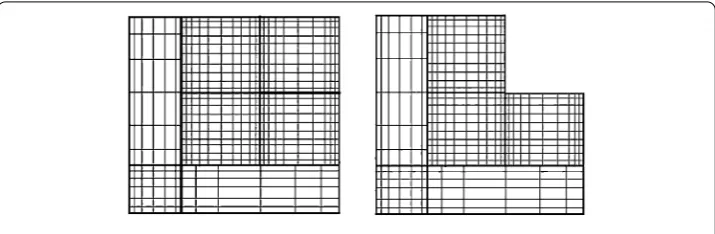
Figure 1The spectral mesh of the domain whenω= 2π(left) andω=3π₂ (right)

We denote that the matrixAis diagonal by block, symmetric, and positive definite. This permits us to solve the problem using the gradient conjugate algorithm method. However, it is not system (18) that we solve since it includes false degrees of freedom. The latter are eliminated by the action of the matrixQT. The global system that we solve is

QTAQ˜ =QTF, (19)

where˜ is the vector formed by the unknowns to internal collocation points and the val-ues of the mortar functions on the skeleton of the decomposition. The matrixA˜ =QTAQ

is symmetric and positive definite. The following conjugate gradient algorithm explains how to solve system (19).

For this, let˜0be arbitrary,R0=QTF–*A˜0,T0=R0, and

αn=

(Rn,Rn)

(Tn,ATn)

,

˜

n+1=˜n+αnTn,

Rn+1=Rn–αnATn,

βn=

(Rn+1,Rn+1) (Rn,Rn)

,

Tn+1=Rn+1+βnTn.

It is clear that all calculations (vector matrix product that is the most expensive, of order

O(N3_{) for each element, as well as projections byQandQ}T_{) are made at the local level}

(on each sub-domain). Consequently, the code can be parallelized.

5.5 Numerical results

We present in this section some numerical tests to confirm the obtained theoretical re-sults. The error between the continuous and discrete solutions is studied. We consider the convergence in the case of both analytical and singular solutions for two domains where ω= 2πandω=3₂π (Fig. 1).

The polynomial degree in the domain¯k, 1≤k≤K, containing the singular point v is

denoted byN. In the other rectangular sub-domains, the degree of the polynomial is fixed less thanN.

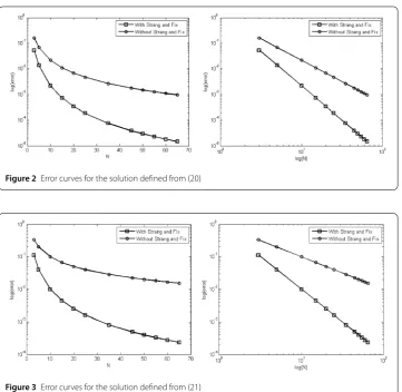
Figure 2Error curves for the solution defined from (20)

Figure 3Error curves for the solution defined from (21)

For the two studied domains, we consider the first singular function as a given solution • forω=3₂π,

ϕ∗_δ(r,θ) =S1(r,θ) =r1.54484φ(θ)

=r1.54484(2.093cos(0.459θ) –cos(1.544θ)

+ 1.0932.193sin(0.459θ) –sin(1.544θ) ), (20)

• ifω= 2π,

ϕ∗_δ(r,θ) =S1(r,θ) =r32

sin3

2θ– 3sin θ 2

+

cos3

2θ–cos θ 2

. (21)

We present in Figs. 2 and 3 the obtained curves of the error respectively for the obtained solution from (20) and (21). The logarithm of the error with respect on one hand toNand on the other hand to the logarithm ofNto obtain the slope is given. The obtained figures show that the Strang and Fix algorithm improves the results.

In the second example we choose the stream function

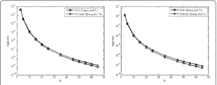
Figure 4Error curves for the solution from (22), forω=3₂π andω= 2π

as an analytic function. In this case, the obtained error curves are presented in Fig. 4 for the two studied domains. We remark that the error is approximately the same. This shows the non-utility of the use of the Strang and Fix algorithm in the case where the solution is regular.

We consider now the second singular function as a given solution which is obtained for each domain:

(i) forω=3π

2 ,

ϕ_δ∗(r,θ) =S2(r,θ) =r1.908529ς(θ)

=r1.908529(4.302cos(0.092θ) –cos(1.908θ)

– 1.81510.869sin(0.092θ) – 0.524sin(1.908θ) ), (23)

(ii) forω= 2π,

ϕ_δ∗(r,θ) =S2(r,θ) =r52

sin5

2θ– 5sin θ 2

+

cos5

2θ–cos θ 2

. (24)

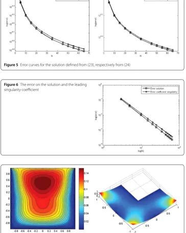
The error convergence curves corresponding to these solutions are presented in Fig. 5. This shows that the convergence is not good with or without the Strang and Fix algorithm. This is due to the fact that we have to add the second singular function to the discrete space

Xδ∗(difficult to numerically implement) in order to improve the convergence.

We study now two examples of the numerical calculation of the discrete leading singu-larity coefficientλ1δwith respect toN.

Example1 ϕ∗_δ(x,y) =sin2πx2sin2πy2andω=3₂π.

N 15 20 25 30 35 40 50

λ1δ 7.0 10–1 4.453 10–3 –0.951 10–9 –3.041 10–12 1.382 10–13 6.221 10–14 0.329 10–14

Example2 ϕ∗_δ(r,θ) =S1(r,θ) =r1.5_{(sin(1.5θ) – 3sin(0.5θ) +cos(1.5θ) –cos(0.5θ)), andω=} 2π.

N 15 20 30 40 45 50 60

Figure 5Error curves for the solution defined from (23), respectively from (24)

Figure 6The error on the solution and the leading singularity coefficient

Figure 7The isovalues of solution for the cavity problem (left) and problem (25) (right)

Figure 6 shows the error curves in a logarithmic scale of the numerical solution of the discrete problem (8) (respectively the leading singularity coefficient) with respect to

log(N) in the case ofω= 2π. Using this figure, the convergence order for the leading sin-gularity coefficient is equal to 1.9986 and is equal to that of the solution. In our precedent work [22], the optimal order of convergence (3.9986) was obtained by the dual method.

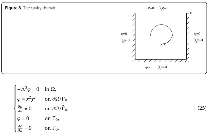
Finally, in Fig. 7 we present an application test corresponding to the discrete solution of the two biharmonic problems:

• problem (25) forω=3₂π,

Figure 8The cavity domain

⎧ ⎪ ⎪ ⎪ ⎪ ⎪ ⎪ ⎪ ⎪ ⎨ ⎪ ⎪ ⎪ ⎪ ⎪ ⎪ ⎪ ⎪ ⎩

–2ϕ= 0 in,

ϕ=x2_y2 _on∂/0,¯

∂ϕ

∂n= 0 on∂/¯0,

ϕ= 0 on0,

∂ϕ

∂n= 0 on0,

(25)

where0={(r,θ) such thatθ= 0 andθ=ω}.

6 Conclusion

In this paper we were interested in the numerical implementation of the mortar spectral method. We considered the biharmonic problem with a homogeneous boundary condi-tion. The Strang and Fix algorithm was implemented. It consists in enlarging the space of the discrete solution by the first singular function. The obtained errors confirm that the used method permits us to improve the order of convergence. The present work shows the importance of the Strang and Fix algorithm coupled with the mortar spectral element method in solving a singular problem in the domain with corner. The mathematical anal-ysis presented in this work can be adapted to other partial differential equations.

Acknowledgements

The authors would like to extend their sincere appreciation to the Deanship of Scientific Research at King Saud University for funding this Research group No (RG-1435-026).

Funding Not applicable.

Availability of data and materials Not Applicable.

Competing interests

The authors declare that they have no competing interests.

Authors’ contributions

The authors declare that the study was realized in collaboration with equal responsibility. All authors read and approved the final manuscript.

Publisher’s Note

Springer Nature remains neutral with regard to jurisdictional claims in published maps and institutional affiliations.

Received: 20 February 2018 Accepted: 14 March 2018 References

1. Baraket, S., R ˘adulescu, V.: Combined effects of concave-convex nonlinearities in a fourth-order problem with variable exponent. Adv. Nonlinear Anal.16(3), 409–419 (2016)

3. Grisvard, P.: Singularities in Boundary Value Problems. Springer, Amsterdam (1982)

4. Kondratiev, V.A.: Boundary value problems for elliptic equations in domain with conical or angular points. Trans. Mosc. Math. Soc.16, 227–313 (1967)

5. Bernardi, C., Maday, Y., Patera, A.T.: A new nonconforming approach to domain decomposition: the mortar element method. In: Brézis, H., Lions, J.L. (eds.) Nonlinear Partial Differential Equations and Their Applications, pp. 16–27 (1991) Collège de France Seminar

6. Babuška, I., Rosenzweig, M.B.: A finite element scheme for domains with corners. Numer. Math.20, 1–21 (1972) 7. Babuška, I., Suri, M.: The optimal convergence rate of the p-version of the finite element method. SIAM J. Numer. Anal.

24, 750–776 (1987)

8. Bernardi, C., Maday, Y.: Polynomial approximation of some singular functions. Appl. Anal.42, 1–32 (1991) 9. Strang, G., Fix, G.J.: An Analysis of the Finite Element Method. Prentice-Hall, New Jersey (1973)

10. Amara, M., Bernardi, C., Moussaoui, M.A.: Handling corner singularities by mortar elements method. Appl. Anal.46, 25–44 (1992)

11. Amara, M., Moussaou, M.A.: Approximation de coefficients de singularité. C. R. Acad. Sci. Paris, Sér. I313, 335–338 (1991)

12. Amara, M., Moussaou, M.A.: Approximation of solution and singularity coefficients for an elliptic equation in a plane polygonal domain. Preprint, E.N.S. Lyon (1989)

13. Kumar, K., Kumar, D., Singh, J.: Fractional modelling arising in unidirectional propagation of long waves in dispersive media. Adv. Nonlinear Stud.5(4), 383–394 (2016)

14. Belhachmi, Z.: Méthode d’éléments spectraux avec joints pour la résolution de problèmes d’ordre quatre. Ph.D. thesis, Université Pierre et Marie Curie (1994)

15. R ˘adulescu, V., Repovš, D.: Partial Differential Equations with Variable Exponents: Variational Methods and Qualitative Analysis. Taylor and Francis Group, Boca Raton (2015)

16. R ˘adulescu, V.: Nonlinear elliptic equations with variable exponent: old and new. Nonlinear Anal., Theory Methods Appl.121, 336–369 (2015)

17. Bernardi, C., Maday, Y.: Approximations Spectrales de Problèmes aux Limites Elliptiques. Collection Mathématiques et Applications. Springer, Paris (1996)

18. Abdelwahed, M., Chorfi, N., R ˘adulescu, V.: Handling geometric singularity by mortar spectral elements method for a fourth order problem. Electron. J. Differ. Equ.2017, 82 (2017)

19. Belhachmi, Z.: Nonconforming mortar element methods for the spectral discretization of two-dimensional fourth-order problems. SIAM J. Numer. Anal.34, 1545–1573 (1997)

20. Anagnostou, G.: Non conforming sliding spectral element methods for unsteady incompressible Navier–Stokes equation. Ph.D. thesis, Maassachusets Institute of Technology, Cambridge (1991)

21. Belhachmi, Z., Bernardi, C.: Resolution of fourth-order problems by the mortar element method. Comput. Methods Appl. Mech. Eng.116, 53–58 (1994)