R E S E A R C H
Open Access
Numerical analysis of unsteady MHD flow
near a stagnation point of a two-dimensional
porous body with heat and mass transfer,
thermal radiation, and chemical reaction
Stanford Shateyi
1*and Gerald Tendayi Marewo
2*Correspondence:
stanford.shateyi@univen.ac.za
1Department of Mathematics,
University of Venda, P Bag X5050, Thohoyandou, 0950, South Africa Full list of author information is available at the end of the article
Abstract
The problem of unsteady MHD flow near a stagnation point of a two-dimensional porous body with heat and mass transfer in the presence of thermal radiation and chemical reaction has been numerically investigated. Using a similarity
transformation, the governing time-dependent boundary layer equations for the momentum, heat and mass transfer were reduced to a set of ordinary differential equations. This set of ordinary equations were then solved using the spectral local linearization method together with the successive relaxation method. The study made among others the observation that the local Sherwood number increases with increasing values of the unsteadiness parameter and the Schmidt number. The fluid temperature was found to be significantly reduced by increasing values of the Prandtl number and the thermal radiation parameter. The velocity profiles were found to be reduced by increasing values of the chemical reaction and the Schmidt number as well as by the magnetic parameter.
1 Introduction
Uniform fluid flow over bodies of various geometries has been considered by many re-searchers over the years due to their numerous applications in industry and engineering. Due to complexity and non-linearity of the modeling governing equations exact solutions are difficulty to obtain. To that end, many researchers have employed different analytical and numerical methods. In recent years, the study of stagnation flow has gained tremen-dous research interest. Stagnation flow is the fluid motion near the stagnation point. The fluid pressure, and the rates of heat and mass transfer are highest in the stagnation area. A flow can be stagnated by a solid wall or a free stagnation point or a line can exist in the interior of the fluid domain. The study of stagnation point flow was pioneered by Hiemenz in []. Wang [] investigated the stagnation flow toward a shrinking sheet and found that the convective heat transfer decreases with the shrinking rate due to an increase in the boundary layer thickness. Motsaet al.[] studied the Maxwell fluid for two-dimensional stagnation flow toward a shrinking sheet. Shateyi and Makinde [] investigated the steady stagnation point flow and heat transfer of an electrically conducting incompressible vis-cous fluid with convective boundary conditions.
The study of heat generation or absorption in moving fluids is of great importance in problems dealing with chemical reactions and those concerned with dissociating fluids. Heat generation effects may alter the temperature distribution and consequently, the par-ticle deposition rate in nuclear reactors, electronic chips. Chamkha and Ahmed [] studied the problem of MHD heat and mass transfer by mixed convection in the forward stagna-tion region of rotating sphere in the presence of heat generastagna-tion and chemical reacstagna-tion effects. Bararniaet al.[] investigated analytically the problem of MHD natural convec-tional flow of a heat generation fluid in a porous medium.
Fluid flows with chemical reaction have key importance in many processes such as dry-ing evaporation at the surface of a water body, energy transfer in a wet cooldry-ing electric power, food processing, groves of fruit trees,etc. The molecular diffusion of species in the presence of a chemical reaction within or at the boundary layer always exists during sev-eral practical diffusive operations. Sevsev-eral researchers have studied flows with chemical reaction reactions. Pal and Talukdar [] presented the combined effects of Joule heating and a chemical reaction on unsteady MHD mixed convection with viscous dissipation over a vertical plate in the presence of a porous medium and thermal radiation. Hayatet al.[] examined the mass transfer effect on unsteady three-dimensional flow of a coupled stress fluid over a stretching surface with chemical reaction. Najibet al.[] investigated the stag-nation point flow and mass transfer with a chemical reaction past a stretching shrinking cylinder.
Unsteady mixed convection flows do not necessarily possess similarity solutions in many practical applications. The unsteadiness and non-similarity in such flows may be due to the free stream velocity or due to the curvature of the body or due to the surface mass transfer or even possibly due to all these effects. Many investigators have confined their studies to either steady non-similar flows or to unsteady semi-similar flows because of the math-ematical difficulties involved in obtaining non-similar solutions for such problems. Patil et al.[] numerically studied the combined effects of thermal radiation and Newtonian heating on unsteady mixed convection flow along a semi-infinite vertical plate. Admon et al.[] studied the behavior of unsteady free convection of a viscous and incompress-ible fluid in the stagnation point region of a heated three-dimensional body considering the temperature-dependent internal heat generation. Ahmad and Nazar [] investigated the unsteady MHD mixed convection boundary layer flow of a viscoelastic fluid near the stagnation point for a vertical surface. Chamkha and Ahmed [] investigated the effects of heat generation/absorption and chemical reaction on unsteady MHD flow heat and mass transfer near a stagnation point of three-dimensional porous body in the presence of a uniform magnetic field.
Rashidi [] presented an analytical solution for three-dimensional steady flow of a con-densation film on an inclined rotating disk by the optical homotopy analysis method. Basiri Parsaet al. [] applied the semi-numerical techniques known as the optimal analysis method (HAM) and the Differential Transform Method (DTM) to study the magneto-hemodynamic laminar viscous flow of a conducting physiological fluid in a semi-porous channel under a transverse magnetic field. Recently Khanet al.[] studied the numerical simulation for unsteady MHD flow and heat transfer of a couple stress fluid over a rotating disk.
The present study aims to investigate the combined effects of thermal radiation, heat generation, viscous dissipation, and chemical reaction on an unsteady mixed convection flow near a stagnation point of two-dimensional porous body. The unsteadiness is induced due to the time-dependent moving plate velocity as well as by the free stream velocity. The paper seeks to compare the performance of two recently developed methods, namely the spectral local linearization method (SLLM) and the spectral relaxation method (SRM). The results generated from these two methods are also validated against the Matlabbvpc routine technique.
2 Mathematical formulation
We consider unsteady laminar incompressible boundary layer flow of a viscous electrically conducting fluid at a two-dimensional stagnation point with magnetic field, thermal radi-ation, heat generation/absorption and suction/injection effects. It is assumed that near the stagnation point the free stream temperature is constant and a uniform transverse mag-netic field is applied normal to the body surface. The fluid properties are assumed to be constant and a uniform chemical reaction is taking place within the flow. Following Eswara and Nath [], the velocity components of the inviscid flow over the two-dimensional body surface are given by
ue(x,t) = ax
( –λτ), ve(x,t) = by
( –λτ). ()
We also assume that near the stagnation point, the free stream temperature and concen-tration are constant. We note that forTw>T∞and/orCw>C∞the buoyancy forces, will aid the flow. On the other hand, forTw<T∞and/orCw<C∞, the resulting buoyancy force
will oppose the forced flow. Under these assumptions as well as the Boussinesq approxi-mation, and following Chamkha and Ahmed [], the governing equations for the current study are given by
∂u
∂x +
∂v
∂y= , ()
∂u
∂t +u
∂u
∂x+v
∂u
∂y=
∂ue
∂t +ue
∂ue
∂x +ν
∂u
∂y – σB
ρ (u–ue)
+gβ(T–T∞) +gβc(C–C∞)x
l, ()
∂T
∂t +u
∂T
∂x +v
∂T
∂y = k
ρcp
∂T
∂y + μ ρcp
∂u
∂y
–
ρcp
∂qr
∂y ± Q ρcp
(T–T∞), ()
∂T
∂t +u
∂C
∂x +v
∂C
∂y =D
∂C
The initial and boundary conditions are
t= :u(x,y,t) =ui(x,y), v(x,y) =vi(x,y), T(x,y,t) =Ti(x,y),
C(x,y,t) =Ci(x,y),
t> :u(x,y,t) = , v(x,y,t) =Vw, T(x,y,t) =Tw,
C(x,y,t) =Cw, aty= ,
t> :u=ue(x,y,t), v=ve(x,y,t), T(x,y,t) =T∞,
C(x,y,t) =C∞, asy→ ∞.
()
3 Similarity analysis
We assume that the velocity varies inversely as a linear function of time making it possible to transform equations ()-() into a set of self-similar equations.
Applying the dimensionless quantities
η=
a
ν( –λτ)
y, τ=at, u= ax
( –λτ)f
(η),
v= –
aν
( –λτ)
f(η), θ(η) = T–T∞ Tw–T∞
, φ(η) = C–C∞ Cw–C∞
()
to ()-() yields the following similarity equations:
f+ff–λη f
–λf–f–Mf– +λ
θ+λφ+ (λ+ ) = , ()
+ R PrR
θ+
f–λη
θ+δθ+Ecf= , ()
Scφ
+f–λη
φ–γ φ= , ()
where M=σB/ρa is the magnetic field parameter, λ is the unsteadiness parameter,
λ=Gr/Rel,λ=Grc/Rel are the buoyancy parameters,Pr=μcp/kis the Prandtl
num-ber,Gr=gβl(Tw–T∞)/νis the Grashof number,Grc=gβl(Cw–C∞)/νis the mod-ified Grashof number,Rel=al/νis the Reynolds number,δ=Q/ρcpais the heat gen-eration/absorption parameter, Ec=νax/cp( –λτ)(Tw–T∞),Sc=ν/Dis the Schmidt number,γ=kr
a( –λτ).
The transformed boundary conditions () become
f() =fw, f() = , θ() = , φ() = , ()
f→, θ→, φ→ asη→ ∞, ()
wherefw= –Vw(( –λτ)/aν)
4 Methods of solution
4.1 Spectral local linearization method (SLLM)
.. Basic idea
Letr= , , , . . . . Suppose thatr+ iterations of the SLLM have been used to solve a given a system of differential equations such as equations ()-(). Also, suppose that each equation can be written in the form
L|r++N|r+=H, ()
whereLandNare the linear and non-linear components, respectively, andHis a given function ofη. Letwbe then-tuple consisting of independent variablezand its derivatives. If we assume thatNis a function ofwonly, then equation () may be replaced with the linearized form
L|r++N|r+∇N|r·(wr+–wr) =H, ()
which shall be solved using the Chebyshev Spectral Collocation Method []. We chose this method due to its ease of implementation and relatively high rate of convergence.
.. Application
Upon using the transformationp=f, equations () and () become
p+fp–λη
p
–λp–p–M(p– ) +λ
θ+λφ+ (λ+ ) = , ()
+ R PrR
θ+
f–λη
θ+δθ+Ecp= , ()
but equation () remains unchanged.
Equation () may be written in the same form as equation () with
L=p–λη
p
– (λ+M)p+λ
θ+λφ+ (λ+ ), ()
Np,p=fp–p and H= –M. ()
The corresponding linearized form () is
L|r++ ∂N
∂p
rpr++
∂N ∂p rp
r+=H+ ∂N
∂p
rpr+
∂N ∂p rp
r–N|r, ()
which upon making use of equations () and (), and simplifying becomes
pr+–λη
p
r+– (λ+M)pr++λθr++λφr+– prpr++frpr+
= –M–pr– (λ+ ). ()
Similarly, equations () and () yield
+ R PrR
θr+–λη
θ
r++δθr++frθr+= –Ecp
Scφ
r+–λ η
φ
r+–γ φr++frφr+= . ()
Before we solve iterative equations (), (), and () for eachr= , , , . . . , we take the following preliminary steps.
. The infinite interval[,∞)on theηaxis is replaced by the finite interval[,L],
whereLis sufficiently large.
. The truncated problem domain[,L]on theηaxis is mapped onto the
computational domain[–, ]on theξ axis.
. The computational domain is partitioned using the Chebyshev collocation points
ξ,ξ, . . . ,ξN, where– =ξN<ξN–<· · ·<ξ= .
For a more detailed explanation of these steps, see for example [] and []. Equations () through () are subject to the boundary conditions
pr+(ξN) = , pr+(ξ) = , ()
θr+(ξN) = , θr+(ξ) = , ()
φr+(ξN) = , φr+(ξ) = , ()
respectively. Applying Chebyshev differentiation [], as done in e.g. [], transforms equations ()-() and ()-(), by the transformationf=pwith boundary condition f() =fw, to the discrete system
Ar+=B, φr+(ξN) = , φr+(ξ) = , ()
Ar+=B, θr+(ξN) = , θr+(ξ) = , ()
Apr+=B, pr+(ξN) = , pr+(ξ) = , ()
Afr+=B, fr+(ξN) =fw, ()
where
A=
ScD
+
–λ
ηI+diag{fr}
D–γI, B=, ()
A=
+ R PrR
D+
–λ
ηI+diag{fr}
D+δI, B= –Ecpr
, ()
A=D+
–λ
ηI+diag{fr}
D– (λ+M)I– diag{pr}, ()
B= –M– (λ+ ) –pr– [λr++λr+], ()
A=D, B=pr+. ()
The solution of each linear system in equations ()-() is preceded by including the corresponding boundary conditions. We do this in the same manner as []. For example, the linear system in equation () becomes
⎛ ⎜ ⎜ ⎝ · · · A · · · ⎞ ⎟ ⎟ ⎠ ⎛ ⎜ ⎜ ⎜ ⎝
φr+(ξ)
.. .
Equations () and () are modified in a similar manner, while equation () becomes
⎛ ⎜ ⎜ ⎝ A
· · · ⎞ ⎟ ⎟ ⎠ ⎛ ⎜ ⎜ ⎝
fr+(ξ)
.. .
fr+(ξN) ⎞ ⎟ ⎟ ⎠= ⎛ ⎜ ⎜ ⎝B
fw ⎞ ⎟ ⎟ ⎠.
The SLLM is driven by initial approximations
f(η) =η+e–η+fw– ,
p(η) = –e–η,
θ(η) =φ(η) =e–η,
which are chosen so that they satisfy boundary conditions () and (). Successive appli-cation of the SLLM generates approximationsfr+,pr+,θr+,φr+for eachr= , , , . . . .
4.2 Successive relaxation method (SRM)
Just like the SLLM, the SRM also makes use of the transformationp=fon the governing equations ()-(). Hence, we begin with the transformed equations () and (), and equation (), which is invariant under this transformation.
As done in [] and [], we proceed in a manner similar to the Gauss-Seidel method for solving a linear system. Consequently, we replace the transformationp=fand equations (), (), and () with the iterative equations
fr+=pr, ()
pr++
fr+–λ η
pr+– (λ+M)pr+=pr–M– (λθr+λφr) – (λ+ ), ()
+ R PrR
θr++
fr+–λ η
θr++δθr++Ecpr+= , ()
Scφ
r++
fr+–λ η
φr+–γ φr+= , ()
subject to boundary condition
fr+(ξN) =fw, ()
and boundary conditions ()-(), respectively.
Just like with the SLLM, we use Chebyshev differentiation to replace equations () through () with the discrete form
Afr+=B, fr+(ξN) =fw, ()
Apr+=B, pr+(ξN) = , pr+(ξ) = , ()
Ar+=B, θr+(ξN) = , θr+(ξ) = , ()
where
A=D, B=pr, ()
A=D+diag{fr+}D–λ η
D– (λ+M)I,
B=pr–M– (λr+λr) – (λ+ ),
()
A=
+ R PrR
D+diag{fr+}D–λη
D+δI, B= –Ecp
r+
, ()
A=
ScD
+diag{f
r+}D–λ η
D–γI, B=. ()
Just like with the SLLM, the following steps are done in a similar manner for the SRM: • For each linear system in equations ()-(), include the corresponding boundary
conditions.
• Choose suitable initial approximationsf,p,θ,φrequired by the SRM to generate
subsequent approximationsfr+,pr+,θr+,φr+for eachr= , , , . . ..
5 Results and discussion
In this section we present a comprehensive numerical parametric study is conducted and the results are reported graphically and in tabular form. Numerical simulations were car-ried out to obtain approximate numerical values of the quantities of engineering interest. The quantities are the surface shear stressf(), surface heat transferθ(), and surface mass transferφ(). In both the SLLM and the SRM numerical simulations, a finite compu-tational value ofη∞= was chosen in theηdirection. This was reached through numer-ical experimentations. This value was found to give accurate results for all the governing physical parameters and beyond the value, the results did not change within prescribed significant accuracy. The number of collocation points used in both SLLM and SRM was Nx= in all the cases considered in this investigation. We set our tolerance level to be
ε= –which we regard to be good enough for any engineering numerical approxima-tion.
We compare the performance of the two methods against each other as well as to the bvpcmethod. Table displays the results generated by the three methods. When varying the magnetic fields strength, it can be clearly observed in the table that, for the current problem, the SLLM is superior to both the SRM and thebvpcmethods.
Table 1 Comparison of the SLLM results off(0) with those obtained by SRM as well as by
bvp4cfor different values of the magnetic parameterM, withλ= 0.5;R= 1;Pr= 0.71;λ1= 0.5;
λ2= 0.5;Ec= 0.1;γ = 0.1;δ= 0.1;fw= 0.5;Sc= 0.22
SLLM SRM bvp4c
M it time (sec) f(0) it time (sec) f(0) time (sec) f(0)
1 9 1.37 2.48466051 34 3.74 2.48466051 15.27 2.48466051
3 8 0.74 2.88909949 21 3.32 2.88909949 17.86 2.88909949
5 8 0.96 3.24098431 17 2.81 3.24098431 18.53 3.24098431
10 7 0.82 3.98172655 13 1.76 3.98172655 18.37 3.98172655
Table 2 Effect of the magnetic parameter onf(0), –θ(0), –φ(0) withλ= 0.5;R= 1;Pr= 0.71;
λ1= 0.5;λ2= 0.5;Ec= 0.1;γ= 0.1;δ= 0.1;fw= 0.5;Sc= 0.22
M f(0) –θ(0) –φ(0)
0 2.25937547 0.37888463 0.49382391 2 2.69541174 0.37785044 0.49091212 5 3.24098431 0.37663629 0.48843976
Table 3 Effect of the transpiration parameterfwonf(0), –θ(0), –φ(0) withλ= 0.5;R= 1;
Pr= 0.71;λ1= 0.5;λ2= 0.5;Ec= 0.1;γ = 0.1;δ= 0.1;M= 2;Sc= 0.22
fw f(0) –θ(0) –φ(0)
–0.5 2.12463544 0.18753160 0.36279720 0.0 2.39659776 0.27651084 0.42802020 0.5 2.69541174 0.37785044 0.49091212 1.0 3.01855731 0.48914126 0.56352188
Table 4 The influence of the heat generation/absorption parameterδonf(0), –θ(0), –φ(0) withλ= 0.5;R= 1;Pr= 0.71;λ1= 0.5;λ2= 0.5;Ec= 0.1;γ = 0.1;M= 2;fw= 0.5;Sc= 0.22
δ f(0) –θ(0) –φ(0)
–0.5 2.67966177 0.56304464 0.48999569 0.0 2.71117974 0.41294180 0.49072523 0.5 2.74660998 0.13156107 0.49424792
while both the heat and the mass transfer on the surface are reduced. Physically, the ap-plication of a magnetic field in the normal direction to the flow produces a drag force which tend to retard the fluid flow velocity, thus increasing the temperature and mass distribution within the fluid flow. In Table , we display the influence of the transpiration parameterfwon the skin friction, the Nusselt number and the Sherwood number. Blowing fluid, withfw< , into the system reduces these three physical quantities whereas sucking fluid,fw> , out of the system increases the three physical quantities under consideration. Generating heat within the flow system significantly affects the heat transfer on the sur-face. The Nusselt number is greatly reduced as heat is generated, but the skin friction as well as the Sherwood number is increased as the heat is generated. These can easily be seen on Table .
Table displays the effect of the unsteadiness parameterλon the shear surface stress, heat transfer on the surface and mass transfer. We consider the accelerating cases only,
Table 5 The influence of the unsteadiness parameterλonf(0), –θ(0), –φ(0) withδ= 0.1;
R= 1;Pr= 0.71;λ1= 0.5;λ2= 0.5;Ec= 0.1;γ = 0.1;M= 2;fw= 0.5;Sc= 0.22
λ f(0) –θ(0) –φ(0)
0 2.61770412 0.44070738 0.52781664 0.5 2.69541174 0.37785044 0.49091212 1.0 2.77234572 0.30219385 0.45252502 1.5 2.84976599 0.20022768 0.41157441
Table 6 The effect of the temperature buoyancy parameterλ1onf(0), –θ(0), –φ(0) with
δ= 0.1;R= 1;Pr= 0.71;λ= 0.5;λ2= 0.5;Ec= 0.1;γ = 0.1;M= 2;fw= 0.5;Sc= 0.22
λ1 f(0) –θ(0) –φ(0)
–0.5 2.23773235 0.36058187 0.52781664 0.0 2.46917284 0.36975021 0.49091212 0.5 2.69541174 0.37785044 0.45252502
Table 7 The influence of the Eckert numberEconf(0), –θ(0), –φ(0) withδ= 0.1;R= 1;
Pr= 0.71;λ= 0.5;λ1= 0.5;λ2= 0.5;γ = 0.1;M= 2;fw= 0.5;Sc= 0.22
Ec f(0) –θ(0) –φ(0)
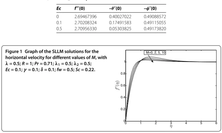
0 2.69467396 0.40027022 0.49088572 0.1 2.70208324 0.17491583 0.49115055 0.5 2.70956330 0.05303825 0.49173820
Figure 1 Graph of the SLLM solutions for the horizontal velocity for different values ofM, with
λ= 0.5;R= 1;Pr= 0.71;λ1= 0.5;λ2= 0.5; Ec= 0.1;γ= 0.1;δ= 0.1;fw= 0.5;Sc= 0.22.
Table displays the effect of temperature buoyancy parameterλon the skin friction,
Nusselt number and Sherwood number. As expected, buoyancy has significant effect on the flow properties. The skin friction increases as the values of the buoyancy parameters are increased. Also the rate of mass transfer at the surface increases as the buoyancy pa-rameters increase, however, the rate of heat transfer decreases with increasing values of the buoyancy parameters.
Figure 2 Graph of the SLLM solutions for the horizontal velocity for different values ofδ, with
λ= 0.5;R= 1;Pr= 0.71;λ1= 0.5;λ2= 0.5; Ec= 0.1;γ= 0.1;M= 0.5;fw= 0.5;Sc= 0.22.
Figure 3 Graph of the SLLM solutions for the horizontal velocity for different values ofλ, with fw= 0.5;R= 1;Pr= 0.71;λ1= 0.5;λ2= 0.5; Ec= 0.1;γ= 0.1;M= 0.5;fw= 0.5;Sc= 0.22.
Figure 4 The influence of the chemical reaction parameter on the horizontal velocity for with
λ= 0.5;R= 1;Pr= 0.71;λ1= 0.5;λ2= 0.5; Ec= 0.1;δ= 0.1;M= 0.5;δ= 0.1;Sc= 0.22.
drag-like force called the Lorentz force. This force tends to cause deceleration in the fluid motion and, therefore, the velocity profiles decrease with increasing values of the magnetic field strength field parameter.
In Figure we display the influence of the heat generation parameter on the velocity distribution. Heating the fluid lightens the fluid particles reducing the friction within the particle interactions thereby increasing the flow velocity as can be clearly seen on Figure . The effect of the unsteadiness parameter on the velocity profiles is displayed in Figure . We observe that near the wall surface, the velocity rapidly increases toward the free stream value. Stretching the sheet accelerates the flow velocity as can be observed in this figure.
Figure 5 Graph of the SLLM solutions for the horizontal velocity for different values ofλ1, withfw= 0.5;R= 1;Pr= 0.71;λ= 0.5;λ2= 0.5; Ec= 0.1;γ= 0.1;M= 0.5;fw= 0.5;Sc= 0.22.
Figure 6 The influence of the chemical reaction parameter on the horizontal velocity for with
λ= 0.5;R= 1;Pr= 0.71;λ1= 0.5;λ2= 0.5; Ec= 0.1;δ= 0.1;M= 0.5;δ= 0.1;Sc= 0.22.
Figure 7 Graph of the SLLM solutions of the temperature profiles for different values ofδ, withλ= 0.5;R= 1;Pr= 0.71;λ1= 0.5;λ2= 0.5; Ec= 0.1;γ= 0.1;M= 0.5;δ= 0.1;Sc= 0.22.
figure that in the current study, the chemical reaction parameter has very little influence on the velocity profiles.
Figure shows the effect of the temperature buoyancy parameterλ, on the velocity
profiles. Increasing the values of the buoyancy parameter leads to the increase of tem-perature gradient. This in turn cause the increases in the values of the velocity profiles as more forces are added with this increase in buoyancy parameters.
In Figure , we display the effect of the Schmidt number on the velocity profiles. Increas-ing the values of the Schmidt numbers implies that the mass concentration becomes more dense. With all other parameters kept constant, increasing the Schmidt number reduces the flow velocity.
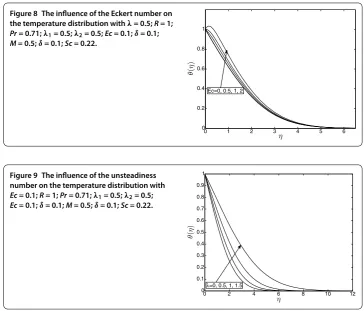
Figure 8 The influence of the Eckert number on the temperature distribution withλ= 0.5;R= 1; Pr= 0.71;λ1= 0.5;λ2= 0.5;Ec= 0.1;δ= 0.1; M= 0.5;δ= 0.1;Sc= 0.22.
Figure 9 The influence of the unsteadiness number on the temperature distribution with Ec= 0.1;R= 1;Pr= 0.71;λ1= 0.5;λ2= 0.5; Ec= 0.1;δ= 0.1;M= 0.5;δ= 0.1;Sc= 0.22.
the presence of the heat source causes great enhancement of the temperature distribution. Therefore heating the fluid flow enhances heat transfer within the fluid flow.
In Figure , we display the influence of the Eckert number on the temperature distri-bution. Increasing the Eckert number allows energy to be stored in the fluid region as a result of dissipation due to viscosity and elastic deformation thus generating heat due to frictional heating. This then causes the temperature within the fluid flow to greatly in-crease.
In Figure , we display the influence of the transpiration parameter on the temperature distribution. As the flow is accelerated due to the increasing values of the transpiration parameter, the temperature profiles are greatly increased.
Figure displays the effects of the thermal buoyancy parameter on the temperature profiles. It is observed that an increase in thermal and solutal Grashof number causes a decrease in the thermal boundary layer thickness, and consequently the fluid tempera-ture decreases due to buoyancy effect. Physically, whenλ/λ(i.e., the buoyancy effect)
increases, the convection cooling effect increases and hence the fluid flow accelerates. Therefore both the temperature and the concentration reduce.
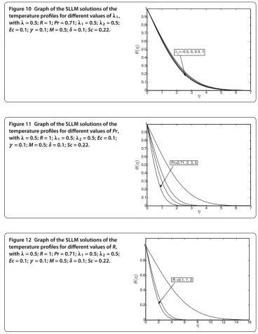
Figure illustrates the effect of increasing the Prandtl number on the temperature pro-files. It can be clearly seen on this figure that increases in Pr bring about a significant de-crease in the fluid temperature. This is expected because the thermal boundary becomes thinner for larger values of the Prandtl number. Therefore, with an increase in the Prandtl number, the rate of thermal diffusion drops.
param-Figure 10 Graph of the SLLM solutions of the temperature profiles for different values ofλ1, withλ= 0.5;R= 1;Pr= 0.71;λ1= 0.5;λ2= 0.5; Ec= 0.1;γ= 0.1;M= 0.5;δ= 0.1;Sc= 0.22.
Figure 11 Graph of the SLLM solutions of the temperature profiles for different values ofPr, withλ= 0.5;R= 1;λ1= 0.5;λ2= 0.5;Ec= 0.1;
γ= 0.1;M= 0.5;δ= 0.1;Sc= 0.22.
Figure 12 Graph of the SLLM solutions of the temperature profiles for different values ofR, withλ= 0.5;R= 1;Pr= 0.71;λ1= 0.5;λ2= 0.5; Ec= 0.1;γ= 0.1;M= 0.5;δ= 0.1;Sc= 0.22.
eter produces a significant decrease in the thermal condition of the fluid flow. This can be explained by the fact that a decrease in the values ofRmeans a decrease in the Rosseland radiation absorptivityk. Thus the divergence of the radiative heat flux decreases ask
increases the rate of radiative heat transferred from the fluid and consequently the fluid temperature decreases.
Figure shows the effect of the chemical reaction parameter on the concentration; physically, as the chemical reaction parameter increases, the concentration profiles de-crease, as can be clearly observed on this figure.
Figure 13 Graph of the SLLM solutions of the concentration profiles for different values ofγ, withλ= 0.5;R= 1;Pr= 0.71;λ1= 0.5;λ2= 0.5; Ec= 0.1;R= 1;M= 0.5;δ= 0.1;Sc= 0.22.
Figure 14 The influence of the unsteadiness number on the concentration distribution with Ec= 0.1;R= 1;Pr= 0.71;λ1= 0.5;λ2= 0.5; Ec= 0.1;δ= 0.1;M= 0.5;δ= 0.1;Sc= 0.22;
γ= 0.1.
Figure 15 The influence of the concentration buoyancy number on the concentration distribution withEc= 0.1;R= 1;Pr= 0.71;
λ1= 0.5;λ= 0.5;Ec= 0.1;δ= 0.1;M= 0.5;δ= 0.1; Sc= 0.22.
Figure depicts the influence of the solutal buoyancy on the concentration profiles. The buoyancy effect slightly reduces the concentration profiles.
Lastly, Figure displays the effect of the Schmidt number on the concentration pro-files. We observe that an increase in the Schmidt number (Sc) decreases the concentra-tion boundary layer thickness. The Schmidt number represents the relative ease of the occurrence of the molecular momentum and the mass transfer and is very important in calculations of the binary mass transfer in multiphase flows.
6 Conclusion
Figure 16 Graph of the SLLM solutions of the concentration profiles for different values ofSc, withλ= 0.5;R= 1;Pr= 0.71;λ1= 0.5;λ2= 0.5; Ec= 0.1;R= 1;M= 0.5;δ= 0.1;γ= 0.1.
into a similar form by applying suitable similarity transformations. The similarity
equa-tions were solved numerically using the spectral local linearization method together with the successive relaxation method. From the numerical results, it is observed that:
. Increasing the values of the magnetic field parameter resulted in increases in the
skin-friction coefficients, whereas the Nusselt number and the Sherwood number and the velocity profiles decrease with increasing values of the magnetic parameter.
. The skin-friction coefficient, the Nusselt number, and the Sherwood number increase with fluid injection.
. The skin-friction coefficients also increase with increasing values of the heat source, the unsteadiness parameter, and the buoyancy parameters as well as the Eckert number.
. The presence of a heat source has significant effects on the Nusselt number as well as on the temperature distribution in the fluid flow.
. The thermal and solutal boundary layer thicknesses increase with increasing values of the unsteadiness parameter and Eckert number but decrease with increasing
values of the buoyancy parameters.
Competing interests
The authors declare that they have no competing interests.
Authors’ contributions
SS formulated, generated and discussed the results and GTM generated the code, discussed the results and proof read the manuscript.
Greek letters
β thermal expansion coefficient
βc compositional expansion coefficient η similarity variable
σ electrical conductivity
λ unsteadiness parameter
λ1,λ2 buoyancy parameters
μ coefficient of viscosity
ν kinematic viscosity
θ dimensionless temperature
Nomenclature
a,b velocity gradient parameters at the boundary layer edge in thex- andy-directions
BO magnetic induction Cf skin-friction coefficient cp heat capacity at constant pressure Ec Eckert number
D mass diffusion
g gravitational acceleration
f dimensionless stream function
kc chemical reaction parameter k thermal conductivity coefficient
M Hartmann number
Pr Prandtl number
R thermal radiation parameter
Q0 heat generation/absorption coefficient
Rel Reynolds number Sc Schmidt number
T temperature
t dimensional time
ue dimensional free stream velocity component inx-direction (u,v) velocity components
(x,y) transverse and normal directions
Author details
1Department of Mathematics, University of Venda, P Bag X5050, Thohoyandou, 0950, South Africa.2Department of
Mathematics, University of Swaziland, Private Bag 4, Kwaluseni, Swaziland, South Africa.
Acknowledgements
The authors wish to acknowledge financial support from the University of Venda and NRF. The authors are very grateful to the reviewers for their constructive suggestions.
Received: 18 August 2014 Accepted: 12 September 2014
References
1. Hiemenz, K: Die Grenzschicht in Einem in Dem Gleichformingen Flussigkeitsstrom Eingetauchten Gerade Kreiszlinder. Dinglers Polytech. J.326, 321-410 (1911)
2. Wang, CY: Stagnation flow towards a shrinking sheet. Int. J. Non-Linear Mech.43, 377-382 (2008)
3. Motsa, SS, Khan, Y, Shateyi, S: A new numerical solution of Maxwell fluid over a shrinking sheet in the region of a stagnation point. Math. Probl. Eng. (2012). doi:10.1155/2012/290615
4. Shateyi, S, Makinde, OD: Hydromagnetic stagnation point flow towards a radially stretching convectively heated disk. Math. Probl. Eng. (2013). doi:10.1155/2013/616947
5. Chamkha, AJ, Ahmed, SE: Unsteady MHD heat and mass transfer by mixed convection flow in the forward stagnation region of a rotating sphere in the presence of chemical reaction and heat source. In: Proceedings of the World Congress on Engineering, WCE, July 6-8, vol. I (2011)
6. Bararnia, H, Ghotbi, AR, Domairry, G: On the analytical solution for MHD natural convection flow and heat generation fluid in porous medium. Commun. Nonlinear Sci. Numer. Simul.14, 2689-2701 (2009)
7. Pal, D, Talukdar, B: Combined effects of Joule heating and chemical reaction on unsteady magnetohydrodynamic mixed convection of a viscous dissipation fluid over a vertical plate in a porous medium with thermal radiation. Math. Comput. Model.54, 3016-3036 (2011)
8. Hayat, T, Awais, M, Safdar, A, Hendi, AA: Unsteady three dimensional flow of couple stress fluid over a stretching surface with chemical. Nonlinear Anal., Model. Control17(1), 47-59 (2012)
9. Najib, N, Bachok, N, Arifin, NM, Ish, A: Stagnation point flow and mass transfer with chemical reaction past a stretching/shrinking cylinder. Sci. Rep.4, 4178 (2014). doi:10.1038/srep04178
10. Patil, PM, Anilkumar, D, Roy, S: Unsteady thermal radiation mixed convection flow from a moving a vertical plate in a parallel free stream: effect of Newtonian heating. Int. J. Heat Mass Transf.62, 534-540 (2013)
11. Admon, MA, Kasim, ARM, Shafie, S: Unsteady free convection flow over a three-dimensional stagnation point with internal heat generation or absorption. World Acad. Sci., Eng. Technol.51, 530-535 (2011)
12. Ahmad, K, Nazar, R: Unsteady magnetohydrodynamic mixed convection stagnation point flow of a viscoelastic fluid on a vertical surface. J. Qual. Meas. Anal.6(2), 105-117 (2010)
13. Chamkha, AJ, Ahmed, SE: Similarity solution for unsteady MHD flow near a stagnation point of a three-dimensional porous body with heat and mass transfer, heat generation/absorption and chemical reaction. J. Appl. Fluid Mech.
4(2)(1), 87-94 (2011)
14. Mahmoud, MAA: Thermal radiation effects on MHD flow of a micropolar fluid over a stretching surface with variable thermal conductivity. Physica A375, 401-410 (2007)
15. Rashidi, MM, Rostami, B, Freidoonimehr, N, Abbasbandy, S: Free Convective heat and mass transfer for MHD fluid flow over a permeable vertical stretching sheet in the presence of the radiation and buoyancy effects. Ain Shams Eng. J. (2014). doi:10.1016/j.asej.2014.02.007
16. Hassan, HN, Rashidi, MM: Analytical solution for three-dimensional steady flow of condensation film on inclined rotating disk by optimal homotopy analysis method. Walailak J. Sci. Technol.10, 479-498 (2013)
18. Khan, NA, Aziz, S, Khan, NA: Numerical simulation for unsteady MHD flow and heat transfer of a couple stress fluid over a rotating disk. PLoS ONE9(5), e95423 (2014). doi:10.1371/journal.pone.0095423
19. Eswara, AT, Nath, G: Effect of large injection rates on unsteady mixed convection flow at a three-dimensional stagnation point. Int. J. Non-Linear Mech.34, 85-103 (1999)
20. Trefethen, LN: Spectral Methods in MATLAB. SIAM, Philadelphia (2000)
21. Shateyi, S, Marewo, GT: A new numerical approach for the laminar boundary layer flow and heat transfer along a stretching cylinder embedded in a porous medium with variable thermal conductivity. J. Appl. Math.2013, Article ID 576453 (2013)
22. Shateyi, S, Marewo, GT: A new numerical approach of MHD flow with heat and mass transfer for the UCM fluid over a stretching surface in the presence of thermal radiation. Math. Probl. Eng.2013, Article ID 670205 (2013)
doi:10.1186/s13661-014-0218-z