Periodic boundary value problems for second-order impulsive integro-differential equations with integral jump conditions

R E S E A R C H

Open Access

Periodic boundary value problems for

second-order impulsive integro-differential

equations with integral jump conditions

Chatthai Thaiprayoon

_{, Decha Samana}

_{and Jessada Tariboon}

*_{Correspondence:}

[email protected]

1_{Department of Mathematics,}

Faculty of Science, King Mongkut’s Institute of Technology Ladkrabang, Bangkok, 10520, Thailand

2_{Centre of Excellence in}

Mathematics, CHE, Sri Ayutthaya Road, Bangkok, 10400, Thailand Full list of author information is available at the end of the article

Abstract

This paper is concerned with the existence of extremal solutions of periodic boundary value problems for second-order impulsive integro-differential equations with integral jump conditions. We introduce a new definition of lower and upper solutions with integral jump conditions and prove some new maximum principles. The method of lower and upper solutions and the monotone iterative technique are used.

MSC: 34B37; 34K10; 34K45

Keywords: impulsive integro-differential equation; lower and upper solutions; periodic boundary value problem; monotone iterative technique

1 Introduction

Differential equations which have impulse effects describe many evolution processes that abruptly change their state at a certain moment. In recent years, impulsive differential equations have become more important tools in some mathematical models of real pro-cesses and phenomena studied in physics, biotechnology, chemical technology, popula-tion dynamics and economics; see [–]. Many papers have been published about exis-tence analysis of periodic boundary value problems of first and second order for impul-sive ordinary or functional or integro-differential equations. We refer the readers to the papers [–]. More recent works on existence results of impulsive problems with integral boundary conditions can be found in [–] and the reference therein. This literature has lead to significant development of a general theory for impulsive differential equations.

The monotone iterative technique coupled with the method of upper and lower solu-tions has been used to study the existence of extremal solusolu-tions of periodic boundary value problems for second-order impulsive equations; see, for example, [–]. This method has been also used to study abstract nonlinear problems; see []. However, in most of these papers concerned with applications of the monotone iterative technique to second-order periodic boundary value problems with impulses, the authors assume that the jump conditions at impulse pointtkof solution values and the derivative of solution values de-pend on the left-hand limits of solutions or the slope of solutions themselves, such as

x(tk) =Ik(x(t–

k)),x(tk) =Ik(x(t–k)),x(tk) =Ik(x(tk–)),x(tk) =Ik(x(t–k)).

In this paper, we consider the periodic boundary value problem for second-order im-pulsive integro-differential equation (PBVP) with integral jump conditions:

⎧ ⎪ ⎪ ⎪ ⎪ ⎪ ⎨ ⎪ ⎪ ⎪ ⎪ ⎪ ⎩

x(t) =f(t,x(t), (Kx)(t), (Sx)(t)), t∈J= [,T],t=tk,

x(tk) =Ik(tk–εk

tk–δk x

_{(s)ds), k= , , . . . ,m,}

x(tk) =I* k(

tk–σk

tk–τk x(s)ds), k= , , . . . ,m, x() =x(T), x() =x(T),

(.)

where  =t<t<t <· · ·<tk <· · ·<tm<tm+=T, f :J×R →Ris continuous ev-erywhere except at{tk} ×R,f(t+k,x,y,z),f(tk–,x,y,z) exist,f(tk–,x,y,z) =f(tk,x,y,z),Ik∈

C(R,R),I*

k∈C(R,R),x(tk) =x(t+k) –x(tk–),x(tk) =x(tk+) –x(tk–), ≤εk≤δk≤tk–tk–, ≤σk≤τk≤tk–tk–,k= , , . . . ,m,

(Kx)(t) =

t



k(t,s)x(s)ds, (Sx)(t) =

T



h(t,s)x(s)ds,

k(t,s)∈C(D,R+_{),h(t,s)∈C(J×J,R}+_{),D={(t,s)∈R}_{, ≤s≤t≤T},R}+_{= [, +∞),k} =

max{k(t,s) : (t,s)∈D},h=max{h(t,s) : (t,s)∈J×J}.

In [, ], the authors discussed some kinds of first-order impulsive problems with the integral jump condition

x(tk) =Ik

tk

tk–τk

x(s)ds–

tk–+σk–

tk–

x(s)ds , (.)

where  <σk–≤(tk–tk–)/, ≤τk–≤(tk–tk–)/,k= , , . . . ,m. We note that the jump condition (.) depends on functionals of path history before impulse pointstkand after the past impulse points tk–. The aim of our research is to deal with the integral jump conditions

x(tk) =Ik

tk–εk

tk–δk

x(s)ds , x(tk) =I_k* tk–σk

tk–τk

x(s)ds , (.)

where ≤εk≤δk≤tk–tk–, ≤σk≤τk≤tk–tk–,k= , , . . . ,m. The integral jump condition (.) means that a sudden change of solution values and the derivative of solution values at impulse pointtkdepend on the area under the curves ofx(t) andx(t) between

t=tk–δktot=tk–εkandt=tk–τktot=tk–σk, respectively. It should be noticed that the impulsive effects of PBVP (.) have memory of the past states.

This paper is organized as follows. Firstly, we introduce a new concept of lower and upper solutions. After that, we establish some new comparison principles and discuss the existence and uniqueness of the solutions for second-order impulsive integro-differential equations with integral jump conditions. By using the method of upper and lower solutions and the monotone iterative technique, we obtain the existence of an extreme solution of PBVP (.). Finally, we give an example to illustrate the obtained results.

2 Preliminaries Let J–_{=J\ {t}

,t, . . . ,tm}, J= [t,t],Jk= (tk,tk+] fork= , , . . . ,m. Let PC(J,R) ={x:

J→R;x(t) is continuous everywhere except for sometkat whichx(tk+) andx(t–k) exist and

x(t–

R) andPC_{(J,R) are Banach spaces with the normsx}

PC=sup{x(t) :t∈J}andxPC=

max{xPC,xPC}. LetE=PC(J,R)∩C(J–,R). A functionx∈Eis called a solution of PBVP (.) if it satisfies (.).

Definition . We say that the functionsα,β∈Eare lower and upper solutions of PBVP (.), respectively, if there existM> ,N≥,L≥,Lk≥,L*k≥, ≤εk≤δk≤tk–tk–, ≤σk≤τk≤tk–tk–, such that

⎧ ⎪ ⎪ ⎪ ⎪ ⎪ ⎨ ⎪ ⎪ ⎪ ⎪ ⎪ ⎩

α_(t)≥f(t,α(t), (Kα)(t), (Sα)(t)) +a(t), t∈J–,

α(tk) =Ik(

tk–εk

tk–δk α

(s)ds) +mk, k= , , . . . ,m,

α_(tk)≥I_k*(tk–σk

tk–τk α(s)ds) +lk, k= , , . . . ,m, α() =α(T),

where

a(t) =

⎧ ⎪ ⎪ ⎨ ⎪ ⎪ ⎩

 ifα_()≥α_(T),

[α_(T)–α_()]

T [ +M[tT–t

_{] +N}t

k(t,s)(sT–s _)ds

+L_Th(t,s)(sT–s_{)ds] ifα}

() <α(T),

mk=

⎧ ⎨ ⎩

 ifα_()≥α_(T),

Lk[α(T)–α()] T

tk–εk

tk–δk(T– s)ds ifα

() <α(T),

lk=

⎧ ⎨ ⎩

 ifα_()≥α_(T),

L*_k[α_(T)–α_()] T

tk–σk

tk–τk (sT–s

_{)ds ifα}

() <α(T), and

⎧ ⎪ ⎪ ⎪ ⎪ ⎪ ⎨ ⎪ ⎪ ⎪ ⎪ ⎪ ⎩

β_(t)≤f(t,β(t), (Kβ)(t), (Sβ)(t)) –b(t), t∈J–,

β(tk) =Ik(

tk–εk

tk–δk β

(s)ds) –m*k, k= , , . . . ,m,

β_(tk)≤Ik*(

tk–σk

tk–τk β(s)ds) –l

*

k, k= , , . . . ,m,

β() =β(T),

where

b(t) =

⎧ ⎪ ⎪ ⎨ ⎪ ⎪ ⎩

 ifβ_()≤β_(T),

[β_()–β_(T)]

T [ +M[tT–t] +N

t

k(t,s)(sT–s)ds

+L_Th(t,s)(sT–s)ds] ifβ_() >β_(T),

m*_k=

⎧ ⎨ ⎩

 ifβ_()≤β_(T),

Lk[β()–β(T)] T

tk–εk

tk–δk(T– s)ds ifβ

() >β(T),

l_k*=

⎧ ⎨ ⎩

 ifβ_()≤β_(T),

L*

k[β()–β(T)] T

tk–σk

tk–τk (sT–s

_{)ds ifβ}

() >β(T).

Lemma . Assume that x∈E satisfies ⎧

⎪ ⎪ ⎪ ⎪ ⎪ ⎨ ⎪ ⎪ ⎪ ⎪ ⎪ ⎩

x(t)≥Mx(t) +N_tk(t,s)x(s)ds+L_Th(t,s)x(s)ds, t∈J–,

x(tk) =Lk

tk–εk

tk–δk x

_{(s)ds, k= , , . . . ,m,}

x(tk)≥L*k

tk–σk

tk–τk x(s)ds, k= , , . . . ,m, x() =x(T), x()≥x(T),

(.)

where M> ,N≥,L≥,Lk≥,L*k≥are constants and≤εk≤δk≤tk–tk–, ≤

σk≤τk≤tk–tk–,k= , , . . . ,m,and they satisfy

_m

k=

Lk(δk–εk) +T

_m

k=

L*_k(τk–σk) + (M+NkT+LhT)T

≤. (.)

Then x(t)≤,t∈J.

Proof Suppose, to the contrary, thatx(t) >  for somet∈J. We divide the proof into two cases:

Case (i). There exists a˜t∈Jsuch thatx(˜t) >  andx(t)≥ for allt∈J. From (.), we havex(t)≥ fort∈J–_{. Sincex(tk)≥L}*

k

tk–σk

tk–τk x(s)ds≥, thenx

_(t)

is nondecreasing in t∈ J and so x()≤x(T). However, by (.) x()≥x(T), then

x() =x(T), which impliesx(t) = constant for allt∈J. Thus,  =x(t)≥Mx(˜t) > , a contradiction.

Case (ii). There existst*_,t

*∈Jsuch thatx(t*) > ,x(t*) < .

Letinft∈Jx(t) = –λ< , then there existst*∈Ji, for somei∈ {, , . . . ,m}, such thatx(t*) = –λorx(t+

i) = –λ. Without loss of generality, we only considerx(t*) = –λ. For the casex(ti+) = –λthe proof is similar. It follows that

x(t)≥Mx(t) +N t



k(t,s)x(s)ds+L T



h(t,s)x(s)ds

≥–λ(M+NkT+LhT), t∈J–,

x(tk)≥L*_k tk–σk

tk–τk

x(s)ds≥–λL*_k(τk–σk), k= , , . . . ,m.

If x(t) >  for allt∈J, thenx(tk) =Lk

tk–εk

tk–δk x

_{(s)ds≥,k= , , . . . ,m. Hence,x(t) is}

strictly increasing onJ, which contradictsx() =x(T). Then there exists a¯t∈Jsuch that

x(¯t)≤.

Let¯t∈Jj,j∈ {, , . . . ,m}. By mean value theorem, we have

xt–_j–λL*_j(τj–σj) –x(¯t)≤x

t+_j–x(¯t) = –x(sj)¯t–t+_j ≤λ(M+NkT+LhT)

_¯

t–t+_j, sj∈(tj,t¯),

xt–_j––λL*_j–(τj––σj–) –x(tj)≤x

t+_j––x(tj) = –x(sj–)

tj–tj+–

≤λ(M+NkT+LhT)

tj–t+j–

, sj–∈(tj–,tj),

xt–_–λL*_(τ–σ) –x(t)≤x

t_+–x(t) = –x(s)

t–t+

≤λ(M+NkT+LhT)

t–t+

, s∈(t,t),

x() –x(t) = –x(s)(t–t)≤λ(M+NkT+LhT)(t–t), s∈(t,t). Summing up the above inequalities, we obtain

x()≤x(¯t) +λ _j

k=

L*_k(τk–σk) + (M+NkT+LhT)(t¯–t)

≤λ _j

k=

L*_k(τk–σk) + (M+NkT+LhT)¯t

. (.)

Lett∈Jh,h∈ {, , . . . ,m}. Ift≤ ¯tby using the method to get (.), then we have

x(t)≤x(t¯) +λ _j

k=h+

L*_k(τk–σk) + (M+NkT+LhT)(¯t–t)

≤λ _m

k=

L*_k(τk–σk) + (M+NkT+LhT)T

.

Ift>¯t, then the above method together with (.), (.) implies that

x(t)≤x(T) +λ _m

k=h+

L*_k(τk–σk) + (M+NkT+LhT)(T–t)

≤x() +λ _m

k=h+

L*

k(τk–σk) + (M+NkT+LhT)(T–t)

≤λ _j

k=

L*_k(τk–σk) + (M+NkT+LhT)¯t

+λ _m

k=h+

L*_k(τk–σk) + (M+NkT+LhT)(T–t)

≤λ _m

k=

L*_k(τk–σk) + (M+NkT+LhT)T

.

Thus,

x(t)≤λ _m

k=

L*_k(τk–σk) + (M+NkT+LhT)T

, t∈J–.

Lett*_∈J

rfor somer∈ {, , . . . ,m}. We first assume thatt*<t*, theni<r. By the mean value theorem, we have

xt*–x(tr) =x

t*–xt+_r+Lr

tr–εr

tr–δr

x(s)ds

=x(sr)t*–t_r++Lr

tr–εr

tr–δr

≤t*–tr

+Lr(δr–εr)

×λ _m

k=

L*_k(τk–σk) + (M+NkT+LhT)T

, sr∈

tr,t*,

x(tr) –x(tr–) =x(tr) –x

t+_r–+Lr–

tr––εr–

tr––δr–

x(s)ds

=x(sr–)

tr–t+r–

+Lr–

tr––εr–

tr––δr–

x(s)ds ≤(tr–tr–) +Lr–(δr––εr–)

×λ _m

k=

L*_k(τk–σk) + (M+NkT+LhT)T

, sr–∈(tr–,tr),

.. .

x(ti+) –x(t*)≤

(ti+–ti) +Li+(δi+–εi+)

×λ _m

k=

L*_k(τk–σk) + (M+NkT+LhT)T

.

Summing up, we get

 <xt*≤–λ+λ _m

k=

Lk(δk–εk) +T

_m

k=

L*_k(τk–σk) + (M+NkT+LhT)T

.

Hence,

_m

k=

Lk(δk–εk) +T

_m

k=

L*_k(τk–σk) + (M+NkT+LhT)T

> ,

which contradicts (.). For the caset*_<t

*, the proof is similar, and thus we omit it. This completes the proof.

Lemma . Assume that x∈E satisfies

x(t)≥Mx(t) +N t



k(t,s)x(s)ds+L T



h(t,s)x(s)ds+[x

_{(T) –x()]}

T

×

 +MtT–t+N t



k(t,s)sT–sds

+L T



h(t,s)sT–sds

, t∈J–,

x(tk) =Lk

tk–εk

tk–δk

x(s)ds+Lk[x

_{(T) –x()]}

T

tk–εk

tk–δk

(T– s)ds, k= , , . . . ,m,

x(tk)≥L*_k tk–σk

tk–τk

x(s)ds+L *

k[x(T) –x()]

T

tk–σk

tk–τk

sT–sds, k= , , . . . ,m,

where M> ,N≥,L≥,Lk≥,L*k≥are constants and≤εk≤δk≤tk–tk–, ≤

σk≤τk≤tk–tk–,k= , , . . . ,m,and they satisfy(.).Then x(t)≤for all t∈J.

Proof Letu(t) = [tT_T–t][x(T) –x()],t∈J, and define

w(t) =x(t) +u(t) =x(t) +

tT–t

T

x(T) –x().

Note thatu() =u(T),u(t)≥ fort∈J. If we prove thatw≤, thenx(t)≤x(t) +u(t)≤ and the proof is complete. Sinceu(t) = [T_T–t][x(T) –x()], then we get

w() =x() +u() =x(T) +u(T) =w(T),

w() =x() +u() =x() +x(T) –x() =x(T),

w(T) =x(T) +u(T) =x(T) –x(T) +x() =x(). Hence,w() >w(T). Indeed, fork= , , . . . ,m,

w(tk) =x(tk) +u(tk)

=Lk

tk–εk

tk–δk

x(s)ds+Lk[x

_{(T) –x()]}

T

tk–εk

tk–δk

T– s ds

=Lk

tk–εk

tk–δk

x(s) +u(s)ds

=Lk

tk–εk

tk–δk

w(s)ds,

and

w(tk) =x(tk) +u(tk)

≥L*_k tk–σk

tk–τk

x(s)ds+L *

k[x(T) –x()]

T

tk–σk

tk–τk

sT–sds

≥L*_k tk–σk

tk–τk

x(s) +u(s)ds

≥L*_k tk–σk

tk–τk

w(s)ds.

Meanwhile, fort=tk,t∈J,

w(t) –Mw(t) –N t



k(t,s)w(s)ds–L T



h(t,s)w(s)ds

=x(t) –Mx(t) –Mt

T

x(T) –x()–N t



k(t,s)x(s)ds–L T



h(t,s)x(s)ds

–[x

_{(T) –x()]}

T

 +MtT–t+N t



k(t,s)sT–sds

+L T



h(t,s)sT–sds

≥.

Consider the linear PBVP

⎧ ⎪ ⎪ ⎪ ⎪ ⎪ ⎨ ⎪ ⎪ ⎪ ⎪ ⎪ ⎩

x(t) =Mx(t) +N_tk(t,s)x(s)ds+L_Th(t,s)x(s)ds–g(t), t∈J–_,

x(tk) =Lk

tk–εk

tk–δk x

_(s)ds+γ

k, k= , , . . . ,m,

x(tk) =L*_ktk–σk

tk–τk x(s)ds+λk, k= , , . . . ,m, x() =x(T), x() =x(T),

(.)

where constantsM> ,N≥,L≥,Lk≥,Lk*≥,γk,λkare constants andg∈PC(J,R), ≤εk≤δk≤tk–tk–, ≤σk≤τk≤tk–tk–,k= , , . . . ,m.

Lemma . x∈E is a solution of(.)if and only if x∈PC(J,R)is a solution of the fol-lowing impulsive integral equation:

x(t) =

T



G(t,s)

g(s) –N

s



k(s,r)x(r)dr–L T



h(s,r)x(r)dr

ds

+ m

k=

–G(t,tk)

L*_k

tk–σk

tk–τk

x(s)ds+λk

+G(t,tk)

Lk

tk–εk

tk–δk

x(s)ds+γk , (.)

where

G(t,s) =

√Me

√

MT_{– }–

⎧ ⎨ ⎩

e√M(T–t+s)_+e√M(t–s)_{, ≤s<t≤T,}

e√M(T+t–s)_+e√M(s–t)_{, ≤t≤s≤T,}

G(t,s) =

e

√

MT_{– }–

⎧ ⎨ ⎩

e√M(T–t+s)_–e√M(t–s)_{, ≤s<t≤T,} –e

√

M(T+t–s)_+e√M(s–t)_{, ≤t≤s≤T.}

This proof is similar to the proof of Lemma . in [], and we omit it.

Lemma . Let M> ,N≥,L≥,Lk≥,L*k≥are constants and≤εk≤δk≤

tk–tk–, ≤σk≤τk≤tk–tk–,k= , , . . . ,m.If

ψ=:  +e

√

MT

√M(e√MT_{– )}

T



N

s



k(s,r)dr+L T



h(s,r)dr

ds+ m

k=

L*_k(τk–σk)

+ 

m

k=

Lk(δk–εk) < , (.)

μ=:  

T



N

s



k(s,r)dr+L T



h(s,r)dr

ds+ m

k=

L*_k(τk–σk)

+

√ M( +e

√

MT₎

(e√MT_{– )} m

k=

Lk(δk–εk) < , (.)

Proof For anyx∈E, we define an operatorFby

(Fx)(t) =

T



G(t,s)

g(s) –N

s



k(s,r)x(r)dr–L T



h(s,r)x(r)dr

ds

+ m

k=

–G(t,tk)

L*_k

tk–σk

tk–τk

x(s)ds+λk

+G(t,tk)

Lk

tk–εk

tk–δk

x(s)ds+γk ,

whereG,Gare given by Lemma .. ThenFx∈PC(J,R) and

(Fx)(t) = –

T



G(t,s)

g(s) –N

s



k(s,r)x(r)dr–L T



h(s,r)x(r)dr

ds

+ m

k=

G(t,tk)

L*_k

tk–σk

tk–τk

x(s)ds+λk

–MG(t,tk)

Lk

tk–εk

tk–δk

x(s)ds+γk .

By computing directly, we have

max

(t,s)∈J×J

G(t,s)

=  +e

√

MT

√M(e√MT_{– )} and

max

(t,s)∈J×J

G(t,s)

= .

On the other hand, forx,y∈PC_{(J,R), we have}

_{(Fx) – (Fy)}

PC =sup t∈J

_{(Fx)(t) – (Fy)(t)}

=sup

t∈J

T



G(t,s)

–N s



k(s,r)x(r) –y(r)dr

–L T



h(s,r)x(r) –y(r)dr

ds

+ m

k=

–G(t,tk)

L*_k

tk–σk

tk–τk

x(s) –y(s)ds

+G(t,tk)

Lk

tk–εk

tk–δk

x(s) –y(s)ds

≤sup

t∈J

T



G(t,s)

Nx(s) –y(s)

s



k(s,r)dr

+Lx(s) –y(s)

T



h(s,r)dr

+ m

k=

G(t,tk)L*k(τk–σk)x(t) –y(t)

+G(t,tk)Lk(δk–εk)x(t) –y(t)

≤ x–yPC

sup

t∈J

T



G(t,s)

N

s



k(s,r)dr

+L T



h(s,r)dr

ds+ m

k=

G(t,tk)L*k(τk–σk)

+G(t,tk)Lk(δk–εk)

≤ψx–y_PC.

Similarly,

(Fx)– (Fy)_PC =sup

t∈J

–

T



G(t,s)

–N s



k(s,r)x(r) –y(r)dr

–L T



h(s,r)x(r) –y(r)dr

ds

+ m

k=

G(t,tk)

L*_k

tk–σk

tk–τk

x(s) –y(s)ds

–MG(t,tk)

Lk

tk–εk

tk–δk

x(s) –y(s)ds

≤sup

t∈J

T



G(t,s)

Nx(s) –y(s)

s



k(s,r)dr

+Lx(s) –y(s)

T



h(s,r)dr

ds

+ m

k=

G(t,tk)L*k(τk–σk)x(t) –y(t)

+MG(t,tk)Lk(δk–εk)x(s) –y(s)

≤ x–yPC

sup

t∈J

T



G(t,s)

N

s



k(s,r)dr

+L T



h(s,r)dr

ds+ m

k=

G(t,tk)L*k(τk–σk)

+MG(t,tk)Lk(δk–εk)

≤μx–yPC.

Thus,

By the Banach fixed-point theorem, F has a unique fixed pointx*_∈PC_{(J,R), and by} Lemma .,x*_{is also the unique solution of (.). This completes the proof.}

3 Main results

In this section, we establish existence criteria for solutions of PBVP (.) by the method of lower and upper solutions and the monotone iterative technique. Forα,β∈E, we write

α≤βifα(t)≤β(t) for allt∈J. In such a case, we denote [α,β] ={x∈E:α(t)≤

x(t)≤β(t),t∈J}.

Theorem . Suppose that the following conditions hold:

(H) αandβare lower and upper solutions for PBVP(.),respectively,such thatα≤β. (H) The functionf satisfies

f(t,x,y,z) –f(t,x,y,z)≤M(x–x) +N(y–y) +L(z–z),

for allt∈J,α(t)≤x≤x≤β(t),(Kα)(t)≤y≤y≤(Kβ)(t),(Sα)(t)≤z≤

z≤(Sβ)(t).

(H) M> ,N≥,L≥,Lk≥,L*_k≥are constants,and≤εk≤δk≤tk–tk–,≤

σk≤τk≤tk–tk–,k= , , . . . ,m,and they satisfy(.), (.)and(.). (H) The functionsIk,I_k*satisfy

Ik

tk–εk

tk–δk

x(s)ds –Ik

tk–εk

tk–δk

y(s)ds =Lk

tk–εk

tk–δk

x(s) –y(s)ds,

I*_k tk–σk

tk–τk

x(s)ds –I_k* tk–σk

tk–τk

y(s)ds ≤L*_k tk–σk

tk–τk

x(s) –y(s)ds,

wheretk–σk

tk–τk α(s)ds≤ tk–σk

tk–τk y(s)ds≤ tk–σk

tk–τk x(s)ds≤ tk–σk

tk–τk β(s)ds,≤σk≤τk≤ tk–tk–,≤εk≤δk≤tk–tk–,k= , , . . . ,m.

Then there exist monotone sequences {αn},{βn} ⊂E which converge in E to the extreme

solutions of PBVP(.)in[α,β],respectively.

Proof For anyη∈[α,β], we consider linear PBVP (.) with

g(t) =ft,η(t), (Kη)(t), (Sη)(t)–Mη(t) –N t



k(t,s)η(s)ds–L T



h(t,s)η(s)ds,

γk=Ik

tk–εk

tk–δk

η(s)ds –Lk

tk–εk

tk–δk

η(s)ds, k= , , . . . ,m,

λk=Ik*

tk–σk

tk–τk

η(s)ds –L*_k tk–σk

tk–τk

η(s)ds, k= , , . . . ,m.

By Lemma ., PBVP (.) has a unique solutionx∈E. We define an operatorAfrom [α,β] toEbyx(t) =Aη(t). We complete the proof in four steps.

Letα=Aαandp=α–α. Thenαsatisfies

α_(t) –Mα(t) –N(Kα)(t) –L(Sα)(t) =ft,α(t), (Kα)(t), (Sα)(t)

–Mα(t) –N(Kα)(t)

–L(Sα)(t), t∈J–,

α(tk) =Lk

tk–εk

tk–δk

α_(s)ds+Ik

tk–εk

tk–δk

α_(s)ds

–Lk

tk–εk

tk–δk

α_(s)ds, k= , , . . . ,m,

α_(tk) =L*_k tk–σk

tk–τk

α(s)ds+Ik*

tk–σk

tk–τk

α(s)ds

–L*_k tk–σk

tk–τk

α(s)ds, k= , , . . . ,m,

α() =α(T), α() =α(T).

We finish Step  in two cases.

Case.α_()≥α_(T), which implies that

a(t) = , α_(t)≥ft,α(t), (Kα)(t), (Sα)(t)

.

Asαis a lower solution of PBVP (.), then fort∈J–,

p(t) –Mp(t) –N(Kp)(t) –L(Sp)(t)

=α_(t) –Mα(t) –N(Kα)(t) –L(Sα)(t) –α_(t) +Mα(t) +N(Kα)(t) +L(Sα)(t)

≥ft,α(t), (Kα)(t), (Sα)(t)

–Mα(t) –N(Kα)(t)

–L(Sα)(t) –f

t,α(t), (Kα)(t), (Sα)(t)

+Mα(t)

+N(Kα)(t) +L(Sα)(t)

= ,

and

p(tk) =α(tk) –α(tk)

=Ik

tk–εk

tk–δk

α_(s)ds –Lk

tk–εk

tk–δk

α_(s)ds–Ik

tk–εk

tk–δk

α_(s)ds

+Lk

tk–εk

tk–δk

α_(s)ds

=Lk

tk–εk

tk–δk

α_(s) –α_(s)ds=Lk

tk–εk

tk–δk

p(s)ds, k= , , . . . ,m,

≥I*_k tk–σk

tk–τk

α(s)ds –L*k

tk–σk

tk–τk

α(s)ds–Ik*

tk–σk

tk–τk

α(s)ds

+L*_k tk–σk

tk–τk

α(s)ds

=L*_k tk–σk

tk–τk

α(s) –α(s)ds=L*k

tk–σk

tk–τk

p(s)ds, k= , , . . . ,m,

p() =α() –α() =α(T) –α(T) =p(T),

p() =α_() –α_()≥α_(T) –α_(T) =p(T).

Then by Lemma .,p(t)≤, which implies thatα(t)≤Aα(t),i.e.,α≤Aα.

Case.α_() <α_(T), which implies that

a(t) = [α

(T) –α()]

T

 +MtT–t+N t



k(t,s)sT–sds

+L T



h(t,s)sT–sds

.

Hence,

p(t) –Mp(t) –N(Kp)(t) –L(Sp)(t) –[p

_{(T) –p()]}

T

 +MtT–t

+N

t



k(t,s)sT–sds+L T



h(t,s)sT–sds

=α_(t) –Mα(t) –N(Kα)(t) –L(Sα)(t) –

[α_(T) –α_()]

T

 +MtT–t

+N

t



k(t,s)sT–sds+L T



h(t,s)sT–sds

–α_(t) +Mα(t) +N(Kα)(t) +L(Sα)(t)

≥ft,α(t), (Kα)(t), (Sα)(t)

–Mα(t) –N(Kα)(t)

–L(Sα)(t) –f

t,α(t), (Kα)(t), (Sα)(t)

+Mα(t) +N(Kα)(t) +L(Sα)(t) = ,

and

p(tk) =α(tk) –α(tk)

=Ik

tk–εk

tk–δk

α_(s)ds +Lk[α

(T) –α()]

T

tk–εk

tk–δk

T– s ds

–Lk

tk–εk

tk–δk

α_(s)ds–Ik

tk–εk

tk–δk

α_(s)ds +Lk

tk–εk

tk–δk

α_(s)ds

=Lk

tk–εk

tk–δk

p(s)ds+Lk[p

_{(T) –p()]}

T

tk–εk

tk–δk

and

p(tk) =α(tk) –α(tk)

≥I_k* tk–σk

tk–τk

α(s)ds +

L*_k[α_(T) –α_()]

T

tk–σk

tk–τk

sT–sds

–L* k

tk–σk

tk–τk

α(s)ds–Ik*

tk–σk

tk–τk

α(s)ds +L*k

tk–σk

tk–τk

α(s)ds

=L*_k tk–σk

tk–τk

p(s)ds+L *

k[p(T) –p()]

T

tk–σk

tk–τk

sT–sds,

k= , , . . . ,m, and

p() =p(T), p() =α_() –α_() <α_(T) –α_(T) =p(T). Then by Lemma .,p(t)≤, which impliesα(t)≤Aα(t),i.e.,α≤Aα.

Step. We prove that ifα≤η≤η≤β, thenAη≤Aη. Letη*

=Aη,η*=Aη, andp=η*–η*, then fort∈J–, and by (H), we obtain

p(t) –Mp(t) –N(Kp)(t) –L(Sp)(t) =ft,η(t), (Kη)(t), (Sη)(t)

–Mη(t) –N(Kη)(t)

–L(Sη)(t) –f

t,η(t), (Kη)(t), (Sη)(t)

+Mη(t) +N(Kη)(t) +L(Sη)(t)

≥ by (H)

.

From (H), we obtain

p(tk) =Lk

tk–εk

tk–δk

p(s)ds, k= , , . . . ,m,

p(tk)≥L*_k tk–σk

tk–τk

p(s)ds, k= , , . . . ,m,

p() =p(T), p() =p(T).

Applying Lemma ., we getp(t)≤, which impliesAη≤Aη.

Step. We show that PBVP (.) has solutions.

Letαn=Aαn–,βn=Aβn–,n= , , . . . . Following the first two steps, we have

α≤α≤ · · · ≤αn≤ · · · ≤βn≤ · · · ≤β≤β, ∀n∈N.

Obviously, eachαi,βi(i= , , . . .) satisfies

α_i(t) –Mαi(t) –N(Kαi)(t) –L(Sαi)(t) =ft,αi–(t), (Kαi–)(t), (Sαi–)(t)

–Mαi–(t) –N(Kαi–)(t)

αi(tk) =Lk

tk–εk

tk–δk

α_i(s)ds+Ik

tk–εk

tk–δk

α_i–(s)ds

–Lk

tk–εk

tk–δk

α_i–(s)ds, k= , , . . . ,m,

α_i(tk) =L*_k tk–σk

tk–τk

αi(s)ds+I_k* tk–σk

tk–τk

αi–(s)ds

–L*_k tk–σk

tk–τk

αi–(s)ds, k= , , . . . ,m,

αi() =αi(T), α_i() =α_i(T), and

β_i(t) –Mβi(t) –N(Kβi)(t) –L(Sβi)(t) =ft,βi–(t), (Kβi–)(t), (Sβi–)(t)

–Mβi–(t) –N(Kβi–)(t)

–L(Sβi–)(t), t∈J–,

βi(tk) =Lk

tk–εk

tk–δk

β_i(s)ds+Ik

tk–εk

tk–δk

β_i–(s)ds

–Lk

tk–εk

tk–δk

β_i–(s)ds, k= , , . . . ,m,

β_i(tk) =L*k

tk–σk

tk–τk

βi(s)ds+Ik*

tk–σk

tk–τk

βi–(s)ds

–L*_k tk–σk

tk–τk

βi–(s)ds, k= , , . . . ,m,

βi() =βi(T), β_i() =β_i(T).

Thus, there existx*andx*such that

lim

i→∞αi(t) =x*(t), ilim→∞βi(t) =x

*_{(t), uniformly ont∈J.}

Clearly,x*,x*satisfy PBVP (.).

Step. We show thatx*,x*are extreme solutions of PBVP (.).

Letx(t) be any solution of PBVP (.), which satisfiesα(t)≤x(t)≤β(t),t∈J. Suppose that there exists a positive integernsuch that fort∈J,αn(t)≤x(t)≤βn(t). Settingp(t) =

αn+(t) –x(t), then fort∈J–,

p(t) =α_n+–x(t)

=Mαn+(t) +N(Kαn+)(t) +L(Sαn+)(t)

+ft,αn(t), (Kαn)(t), (Sαn)(t)–Mαn(t)

–N(Kαn)(t) –L(Sαn)(t)

–ft,x(t), (Kx)(t), (Sx)(t)

–N(Kx)(t) –L(Sx)(t) +ft,αn(t), (Kαn)(t), (Sαn)(t)

–ft,x(t), (Kx)(t), (Sx)(t)–Mαn(t) –x(t)

–NK(αn)(t) – (Kx)(t)–L(Sαn)(t) – (Sx)(t)

≥Mp(t) +N(Kp)(t) +L(Sp)(t),

and

p(tk) =αn+(tk) –x(tk) =Lk

tk–εk

tk–δk

p(s)ds, k= , , . . . ,m,

and

p(tk) =α_n+(tk) –x(tk) =L*_k

tk–σk

tk–τk

αn+(s)ds+Ik*

tk–σk

tk–τk

αn(s)ds

–L*_k tk–σk

tk–τk

αn(s)ds–I_k* tk–σk

tk–τk x(s)ds

≥L*_k tk–σk

tk–τk

αn+(s)ds+L*k

tk–σk

tk–τk

αn(s)ds

–L*_k tk–σk

tk–τk

αn(s)ds–L*_k tk–σk

tk–τk x(s)ds

=L*_k tk–σk

tk–τk

p(s)ds, k= , , . . . ,m,

and

p() =p(T), p() =p(T).

Still by Lemma ., we have for allt∈J,p(t)≤,i.e.,αn+(t)≤x(t). Similarly, we can prove that x(t)≤βn+(t), t∈J. Therefore, αn+(t)≤x(t)≤βn+(t), for all t∈J, which implies

x*(t)≤x(t)≤x*(t). The proof is complete.

4 An example

In this section, in order to illustrate our results, we consider an example.

Example . Consider the following PBVP:

⎧ ⎪ ⎪ ⎪ ⎪ ⎪ ⎪ ⎪ ⎪ ⎪ ⎪ ⎨ ⎪ ⎪ ⎪ ⎪ ⎪ ⎪ ⎪ ⎪ ⎪ ⎪ ⎩

u(t) = _t_{(u(t) – ) +}  [

t

tsu(s)ds] +

[



tsu(s)ds], t∈J= [, ],t=,

u(_) = _    

u(s)ds, k= ,

u( ) =

 

   

u(s)ds, k= ,

u() =u(), u() =u().

Setk(t,s) =t_s_{,h(t,s) =t}_s_{,m= ,t}

=_,δ=_,ε=_,τ=_,σ=_,T= . Obviously,

α= ,β=  are lower and upper solutions for (.), respectively, andα≤β. Let

f(t,x,y,z) =  t

_(x – ) +  y  +  z  , we have

f(t,x,y,z) –f(t,x,y,z)≤ 

(x–x) + 

(y–y) + 

(z–z),

whereα(t)≤x≤x≤β(t), (Kα)(t)≤y≤y≤(Kβ)(t), (Sα)(t)≤z≤z≤(Sβ)(t),t∈J. It is easy to see that

I





 

x(s)ds –I





 

y(s)ds =  

 

 

x(s) –y(s)ds,

and

I*





 

x(s)ds –I*





 

y(s)ds = 

 

 

x(s) –y(s)ds,

whenevertk–σk

tk–τk α(s)ds≤ tk–σk

tk–τk y(s)ds≤ tk–σk

tk–τk x(s)ds≤ tk–σk

tk–τk β(s)ds,k= .

TakingM=_,N=_,L=_,L=_,L*=, it follows that

_m

k=

Lk(δk–εk) +T

_m

k=

L*_k(τk–σk) + (M+NkT+LhT)T

=    –   +     –   +  +   ()() +   ()()  = ≤, and

ψ =  +e

√

MT

√M(e√MT_{– )}

× T  N s 

k(s,r)dr+L T



h(s,r)dr

ds+ m

k=

L*_k(τk–σk)

+  m k=

Lk(δk–εk)

=  +e

 

(_)(e _{– )}

    s 

srdr+ 





srdr

ds+    –   +      –  

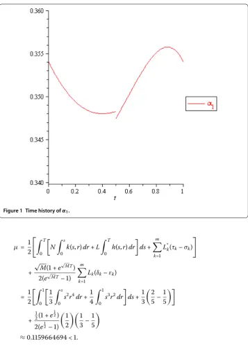
Figure 1 Time history ofα1.

μ=  

T



N

s



k(s,r)dr+L T



h(s,r)dr

ds+ m

k=

L*_k(τk–σk)

+

√ M( +e

√

MT₎

(e√MT_{– )} m

k=

Lk(δk–εk)

=  





 

s



srdr+  





srdr

ds+ 

 –

 

+  ( +e

 )

(e– )

 

 –

 

≈. < .

Therefore, (.) satisfies all the conditions of Theorem .. So, PBVP (.) has minimal and maximal solutions in the segment [α,β].

Substitutingα,βinto monotone iterative scheme, we obtain

⎧ ⎪ ⎪ ⎪ ⎪ ⎪ ⎪ ⎪ ⎪ ⎪ ⎨ ⎪ ⎪ ⎪ ⎪ ⎪ ⎪ ⎪ ⎪ ⎪ ⎩

α_(t) –  α(t) –

 

t t

_s_α

(s)ds–_

 t

_s_α (s)ds = –_t_{, J= [, ],t=}

,

α(_) =_

   

α_(s)ds, k= ,

α_(_) =_    

α(s)ds, k= ,

α() =α(T), α() =α(T),

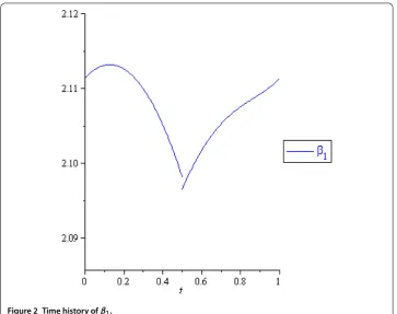
Figure 2 Time history ofβ1.

and

⎧ ⎪ ⎪ ⎪ ⎪ ⎪ ⎪ ⎪ ⎪ ⎪ ⎨ ⎪ ⎪ ⎪ ⎪ ⎪ ⎪ ⎪ ⎪ ⎪ ⎩

β_(t) –_β(t) – _

t

tsβ(s)ds–_



tsβ(s)ds =_t_–

t+  t–



, J= [, ],t=  ,

β(_) =_

   

β_(s)ds, k= ,

β_(_) =_    

β(s)ds, k= ,

β() =β(T), β() =β(T).

(.)

After using the variational iteration method [] for (.), (.), the approximate solutions forαandβcan be illustrated as Figure  and Figure , respectively.

Competing interests

The authors declare that they have no competing interests.

Authors’ contributions

All authors contributed equally in this article. They read and approved the final manuscript.

Author details

1_{Department of Mathematics, Faculty of Science, King Mongkut’s Institute of Technology Ladkrabang, Bangkok, 10520,}

Thailand.2_{Centre of Excellence in Mathematics, CHE, Sri Ayutthaya Road, Bangkok, 10400, Thailand.}3_{Department of}

Mathematics, Faculty of Applied Science, King Mongkut’s University of Technology North Bangkok, Bangkok, 10800, Thailand.

Acknowledgements

This research is supported by the Centre of Excellence in Mathematics, the Commission on Higher Education, Thailand.