Observation of Different Behaviors of Logistic Map for Different Control Parameters

http://www.sciencepublishinggroup.com/j/ijamtp doi: 10.11648/j.ijamtp.20180403.14

ISSN: 2575-5919 (Print); ISSN: 2575-5927 (Online)

Observation of Different Behaviors of Logistic Map for

Different Control Parameters

Musammet Tahmina Akter

1

, Mohammad Abul Mansur Chowdhury

2

1

Department of Mathematics, Chittagong University of Engineering & Technology, Chittagong, Bangladesh

2

Jamal Nazrul Islam Research Center for Mathematical and Physical Sciences, University of Chittagong, Chittagong, Bangladesh

Email address:

To cite this article:

Musammet Tahmina Akter, Mohammad Abul Mansur Chowdhury. Observation of Different Behaviors of Logistic Map for Different Control Parameters. International Journal of Applied Mathematics and Theoretical Physics. Vol. 4, No. 3, 2018, pp. 84-90.

doi: 10.11648/j.ijamtp.20180403.14

Received: October 3, 2018; Accepted: October 18, 2018; Published: December DD, 2018

Abstract:

The logistic map is one of the most important but common examples of chaotic dynamics. The object shows the

crucial belief of the deterministic chaos theory that brings a new procedural structure and apparatus for exploring and understanding complex behavior in dynamical systems. We put an importance on report of the Verhulst logistic map which is one of the potential models and methods for researching dynamical systems that could develop to chaotic. Chaotic signals present a special difficulty in parameter estimation. The difficulty arises from the definition of a chaotic system because of sensitive dependence on initial conditions. It is seen that very slight changes in the initial conditions cause significant effects in the evolution. In general the chaotic systems are nonlinear and apparently random but they are deterministic. The main objective of this paper is how can find the logistic map equation and investigated the chaotic behavior for the logistic equation by varying the control parameters and finally discover Lyaponov exponent, Bifurcation diagrams etc.

Keywords:

Logistic Map, Chaos, Lyapunov Exponent, Bifurcation, Cobweb, Attractor

1. Introduction

The logistic map is a one dimensional discrete time demographic model how very complex, chaotic behavior can arise from very simple non-linear dynamical equations. Mathematically, the logistic map is written as:

x_{n 1+} =rx (1 x )_n − _{n (1)}

Where,

x_n∈[0,1] and represents the ratio of existingpopulation to the maximum possible population at year n and hence x 0

represents the initial ratio of population to maximum (at year 0), r∈ [0,4] _{and represents a combined rate for reproduction and} starvation. It was originally made as a very simple model for the population numbers of species in the presence of limiting factors such as food supply or disease containing two causal loops:

i Due to reproduction the population will increase at a rate proportional to the current population when the population size is small.

ii Due to starvation where the growth rate will decrease

at a rate proportional to the value obtained by taking the theoretical carrying capacity of the environment less the current population.

This type of simple equation already exhibits wonderful dynamics, quickly summarized. In a cobweb plot, the dynamics of the evolution of the map can be seen quickly. The applications of logistic map in engineering and technology are enormous. The focus of paper is on design of a chaotic noise generator governed by a logistic map [1]. The performance evaluation results demonstrate correct operation of the analog noise generating circuit system. Paper examined practical applications of chaos theory in microelectronic field using logistic map. It was found in their study that logistic map modeling is highly promising when genetic algorithm is used for numerical simulations [2]. Moreover, paper has shown that some nonlinear systems that have their sub-domains on the logistic map are often characterized with unique chaotic attractors [3]. These chaotic attractors have interesting stabilizing characteristics. This indeed is a good contribution to the literature on the exciting dynamic of logistic model.

general form of realistic logistic equation can be derived from logistic differential equation. Then we have shown how it matched with bounded population model. Later on we have deduced logistic difference equation from the logistic differential equation which is the logistic map. Lastly, the present paper which is strongly motivated by the quest to introduce the beginners to the theories of chaos and nonlinear dynamics focus on the development of time series and cobweb plot and also bifurcation and Lyapunov exponent based-chaos diagram in one dimensional logistic map.

2. Methodology

We know y=Cekt (2)

is the exponential growth model for unlimited growth. But for physically viable situation we cannot take this type of population model because this will give us unlimited growth of the species. For a realistic case we have to take an account that when we put forward with a population model most often we have to encounter an upper limit to the population which is called the carrying capacity L. This upper limit exists because of some limiting factor in the environment such as food, water, shelter, predation, etc. i.e. if we consider a logistic differential equation model with exponential growth which has some limiting value, say , L and a constant of proportionality, k then we can claim an accepted model.

dy y

ky(1 )

dt = −L (3)

If y is between 0 and L then dy

dt is positive and the

population is increasing. If y is greater than L then dy

dt is

negative and the population is decreasing. Solving the logistic differential equation (3) we can find the logistic equation. After separating the variables, equation (3) can be written as dy kdt y y 1 L =  ₋     

which can be rewritten as

1 1

dy dy kdt

y + L y =

∫ ∫ ∫

− (4)

Integrating and after simplification this becomes

(

)

L y kt C 1 e = _{− +} +

If we put e− =C b then we obtained

L y

kt 1 be

= ₋

+ (5)

Equation (5) is the general form for the logistic equation. If we look very carefully equation (3) it is clear that the general form of the logistic differential equation is

dp ₂

ap bp (a,b o)

dt = − > , (6)

which is a basic model that can describe the behavior of some species population p(t) that is subject to no external influences. Assuming that the actual population of the species can be determined for the current generation, it will be seen that the population at some time n can be predicted solely from the knowledge of the present population. This differential equation can be solved using separation of variables like before. But it will be interesting and more significant if we use numerical method to solve this differential equation. Then with the help of computer we can predict more accurate behavior of the species of population. To use numerical method we can write the derivative term of equation (6) as difference equation. Let us first consider the step size h which designates the time between t0 , t1 , t2 ,…..

tn such that t_{n 1+} =t_n +h

.

_{In the case of population model} h might represent the line between mating seasons, i.e. if p0 is the population at time t0 , then by integration we can predict pn at any later time tn .

Hence, dp pn 1 pn

dt h

− +

= (7)

Using (7) equation (6) can be rewritten as

2 p_{n 1+} =p_n+(ap_n−bp )h_n

p_{n 1+} =p_n+p (ah_n −bh p )_n

p_{n 1+} =p (1 ah_n + −bh p )_n

Now we can let 1 ah+ = r and bh=d reducing the equation to

2

p_{n 1+} =r p_n−d p_n (8)

Substitution of p_n rx_n d =

Equation (8) be comes

x_{n 1+} =r x (1 x )_n − _n (9)

This is a simplified form of the logistic difference equation which we derived from the logistic differential equation which is exactly same as equation (2). The logistic difference equation is that given an initial population x0 ,

x₁=r x (1 x )₀ − ₀

x₂ =r x (1 x )₁ − ₁

………

………

x_n =r x_{n 1−} (1−x_{n 1−} ) ₍₁₀₎

Originally population modeling is extremely complicated but by analyzing the end behavior of the orbits produces by equation (9), the fate of any initial population can be determined. Although the logistic function is a fairly basic equation the mathematics can get rather complicated when computing orbits fate. For this reason our attention will examine for estimating the parameters of chaotic signals of the logistic map. The logistic map has very interesting properties for varying values of the parameter r in (10). Once we have a formula then we can study the behavior of the logistic equation. That means how the behavior changes with the change of the parameter valuer. Here we mentioned that chaos can come into play when the value of r is beyond 2.5. In the following section we will mainly focus on that point for initial condition and for different number of iterations.

3. Result and Discussion

The notion of chaos implies three things: (i) the system is bounded (ii) it is periodic and (iii) has sensitive dependence on initial conditions. Of course boundedness and periodicity are relatively straightforward things to prove. However the dependence on initial conditions is a bit more difficult to show. But graphically this dependency is easy to see. Whenris less than 1 the population will eventually die and also independent of the initial population which is shown in figure 1.

Figure 1. Behaviorforris less than 1 and x∈[0,1].

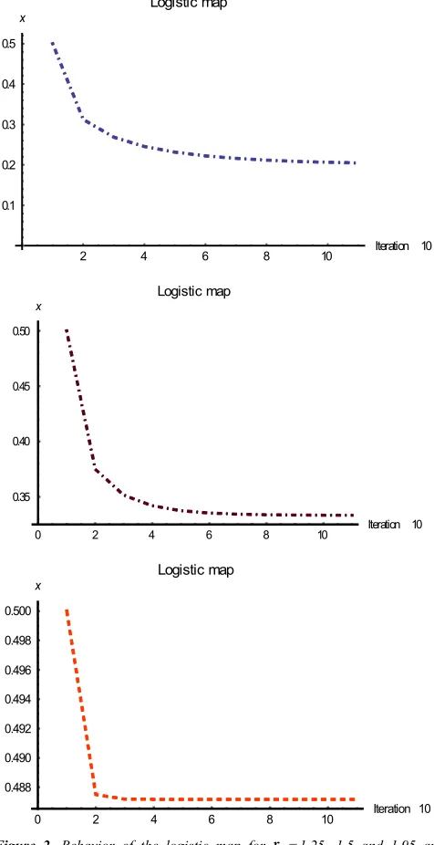
Figure 2. Behavior of the logistic map for r =1.25, 1.5 and 1.95 and

x .5= .

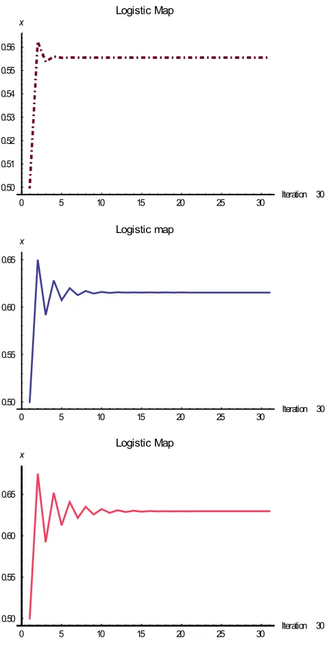
In figure2 when r between 1 and 2 the population will quickly stabilize on a single value and the value depends on parameter r but does not depend on the initial population. When r lies between 2 and 3 the population will also eventually stabilize on a single value but for some times first oscillates around that value. Again, the final value does not depend on the initial population. This case is shown in figure 3.

Whenris 3.45 the population will oscillate between two values forever. These two values are dependent on r but independent of the initial population which is depicted by figure 4.

0.2 0.4 0.6 0.8 1.0

0.05 0.10 0.15 0.20 0.25

f x _.r _0.25

f x _.r _0.75

f x _.r _0.95

f x _.r _0.95

f x _.r _0.99

2 4 6 8 10 Iteration 10

0.1 0.2 0.3 0.4 0.5 x

Logistic map

0 2 4 6 8 10 Iteration 10

0.35 0.40 0.45 0.50 x

Logistic map

0 2 4 6 8 10 Iteration 10

0.488 0.490 0.492 0.494 0.496 0.498 0.500 x

Figure 3. Behavior of the logistic map for

r

=2.25, 2.5 and 2.7 and

x .5= .

Figure 4. Behavior of the logistic map for r =3.45.

When ris 3.45 the population will oscillate between two values forever. These two values are dependent on r but independent of the initial population which is depicted by figure 4. Whenr slightly bigger than 3.54 the population will oscillate between 8 values then 16, 32 etc. which is seen in figure 5. But when r=4and x=.1the behavior of logistic map is chaotic. This type of behavior is seen in figure 6.

Figure 5. Behavior of the logistic map for r =3.56 and x=.001.

Figure 6. Behavior of the logistic map is Chaotic for r = 4 and x=.1.

Finally, if starting value of r>1 but less than 3 successive points flow to a fixed point at a nonzero value of x. However for values ofr a little larger than 3 the fixed point bifurcates to a limit cycle of period 2. This then bifurcates again at a larger value of r to a limit cycle with period 4. As r

increases the period continues to double at successively closer and closer values of r until at around r =4the period becomes infinity and have chaotic behavior.

(i)

0 5 10 15 20 25 30 Iteration 30

0.50 0.51 0.52 0.53 0.54 0.55 0.56 x

Logistic Map

0 5 10 15 20 25 30 Iteration 30

0.50 0.55 0.60 0.65 x

Logistic map

0 5 10 15 20 25 30 Iteration 30

0.50 0.55 0.60 0.65 x

Logistic Map

5 10 15 20 25 Iteration 25

0.2 0.4 0.6 0.8 x

Logistic Map

5 10 15 20 25 30 Iteration 30

0.2 0.4 0.6 0.8 x

Logistic Map

50 100 150 200 250 300 Iteration 300 0.2

0.4 0.6 0.8 1.0 x

Logistic Map

3.6 3.7 3.8 3.9 4.0 r

(ii)

Figure 7. Lyapunov exponent dynamics for (i)r∈[3.5,3.99999] and x=.1 and (ii) r∈[0,4] and x=.1.

All the features and their dynamics can see more easily in the Lyapunov exponent. A defining feature of a chaotic system is sensitivity to initial conditions. If two trajectories which start off close to each other deviate more and more with increasing time the system is said to be chaotic. The rate at which nearby trajectories deviate from each other with time is characterized by a quantity called the Lyapunov exponent. There are a host of estimation schemes to determine the value of the Lyapunov exponent from a time series most of which assume that the initial condition is known. The main significance of these figures are that one can easily distinguish the regions which are chaotic r> 0 from the regions which tend to a fixed point or limit cycle (r< 0). There are several points (the first is at r = 3.0) where the Lyapuov exponent hits 0 and then goes negative again. These are the period doubling bifurcations. Precisely at the period doubling point the system is at the limit of chaos but then becomes non-chaotic when the period doubles. In figure 7(i) for r in the range greater than the point where f(x) first goes positive, there are many regions where f(x) is negative islands of stability where the behavior is fixed point or limit cycle. However in figure 7(ii) at the end of the period doubling regime at r about 3.577, f(x) crosses the axis and the system enters a chaotic region. i.e. This figure shown that chaos emerges (i.e. f(x)> 0) for r between 3.569944 and 3.569948.

(i)

(ii)

(iii)

(iv)

(v)

Figure 8. Graph of (i) f(x) for r= 3.835, x∈[0,1],(ii) f(f(x)) for r= 3.2, [0,1]

x∈ , (iii) [f(x), x, f(f(x))] for x∈[0,1], (iv) f(f(f(x))) for r= 3.96, [0,1]

x∈ , and(v)f(f(f(f(x)))) for r= 4, x∈[0,1] respectively.

1 2 3 4 r

3 2 1 r

0.0 0.2 0.4 0.6 0.8 1.0 x

0.2 0.4 0.6 0.8 1.0 y

0.2 0.4 0.6 0.8 1.0 x

0.2 0.4 0.6 0.8 1.0 y

0.2 0.4 0.6 0.8 1.0 x

0.2 0.4 0.6 0.8 1.0 y

0.2 0.4 0.6 0.8 1.0 x

0.2 0.4 0.6 0.8 1.0 y

0.2 0.4 0.6 0.8 1.0 x

For certain values of r the sequence of xnconverges to a fixed point value x wherex= f x( ). In figure 9 (i) illustrate a fixed point graphically for the case of r= 3.835 . The sequence towards which the x values converge is called an attractor. It will be seen that an attractor may be a fixed point, a limit cycle or a chaotic attractor. But mainly, interested in the nature of the attractor as a function ofr. Fixed-Point gives a result when two successive values are exactly the same. If convergence is very slow or if round off errors prevent exact agreement it is best to put in a less stringent test for determining whether convergence has been reached. A fixed point is stable i.e. it converge towards it if start off not too far away provided f′( ) 1x 〈 . Since f x′( )=r(1 2 )− x , the fixed point at x = 0 is stable when r〈1. For r>1this fixed point is unstable and figure 8 also shown what happens instead.

(i)

(ii)

(iii)

Figure 9. Bifurcation diagram showing the range of behavior for the logistic map at various values of r ,(i) r∈[2.99,4], (ii) r∈[3.2,4] and (iii)

[3,4] r∈ .

This figure just shows the region for r > 2.82 which is the most interesting part. For smaller values of r one always has a fixed point which is at 0 for r < 1and at a non-zero value for 1 < r < 3. This figure just shows the attractors the sets of values of x towards which the iterations converge for different values of r. There can also be unstable fixed points and limit cycles which we don't see. For example the fixed point which is stable for r<3 continues smoothly for r>3 but it becomes unstable so the iterations don't flow towards it and hence it does not appear on the plot for r>3. Instead the stable attractor a length-2 cycle appears in the figure for r just greater than. Figure-10 shows that the cobweb plot for r= 3.88 and x= 0.5 and also have taken 100 iterations.

Figure 10. Cobweb plot showing the iterative behavior of the logistic map in a chaotic region.

4. Conclusion

In this paper, many important features of the simple one dimensional logistic map are preserved in the new dimension and their behavior is analyzed. Logistic map can be utilized to launch interested beginners to the concept of chaos diagram a basic concept in nonlinear dynamics and chaos. Its parameter 3<r<4 investigated by Lyapunov exponent. It is interested to the chaos diagram develop exhibited fractal structures by its layers of order within chaos as can be found in the bifurcation diagrams of nonlinear dynamical systems. The Lyapunov exponent has shown at a glance how the structures and features move in control parameters.

References

[1] Díaz-Méndez A, MarquinaPérez JV, Cruz-Irrison M, Vázquez-Medina R, Del-Río-Correa JL. Chaotic noise MOS generator based on Logistic map. Micro electronics Journal, 2009, 40: 638-640.

[2] Siji PD, Rajesh R Takagi-Sugeno Fuzzy modelling of Logistic map using genetic algorithm. International Journal of Wisdom Based Computing, 2011, 1(3): 9-13.

[3] George M. Stability areas in Logistic map. Advanced Research in Scientific Areas, 2012.

0.2 0.4 0.6 0.8 1.0

0.2 0.4 0.6 0.8 1.0

[4] Wei JG, Leng G. Lyapunov exponent and Chaos of Duffing’s equation perturbed by white noise. Applied Mathematics and Computation, 1997, 88: 77-93.

[5] Kathira M. A Lyapunov exponent approach for identifying chaotic behaviour in a finiteelement based drills string vibration model. A thesis submitted to the office of Graduate Studies of Texas, A & M University in partial fulfillment of the requirements for the degree of Master of Science in Mechanical Engineering, 2009.

[6] Shuichi A, Yoshifumi N. A chaotic cryptosystem using Lyapunov exponent. The 15th IEEE International Workshop on Nonlinear Dynamics of Electronic Systems, 2007, NDE’07Tokushima, Japan.

[7] Andrzej S, Tomasz K. Estimation of the dominant Lyapunov exponent of non-smooth systems on the basis of mass synchronization. Chaos, Solitons and Fractals, 2003; 15: 233-244.

[8] Andrzej S, Artur D, Tomasz K. Evaluation of the largest Lyapunov exponent indynamical systems with time delay. Chaos, Solitons and Fractals, 2005; 23: 1651-1659.

[9] T. A. O. Salau and O. O. Ajide, Development of a Lyapunov Exponent Based Chaos Diagram in the Parameter Plane of Logistic Map, British Journal of Applied Science & Technology, 2014, 4(21): 3096- 3106.

[10] Nandi A. , Dutta D., Bhattacharjee J. K. and Ramaswamy R., 2005, Chaos 15, 023107, DOI: 10.1063/1.1914755.