Free-flow wind speed from a blade-mounted flow sensor

https://doi.org/10.5194/wes-3-121-2018

© Author(s) 2018. This work is distributed under the Creative Commons Attribution 4.0 License.

Free-flow wind speed from a blade-mounted flow sensor

Mads Mølgaard Pedersen1, Torben Juul Larsen1, Helge Aagaard Madsen1, and Søren Juhl Andersen2

1_{Wind Energy Department, Technical University of Denmark, Frederiksborgvej 399, 4000 Roskilde, Denmark} 2_{Wind Energy Department, Technical University of Denmark, Nils Koppels Alle,}

Building 403, 2800 Kgs. Lyngby, Denmark

Correspondence:Mads Mølgaard Pedersen ([email protected])

Received: 15 December 2017 – Discussion started: 2 January 2018

Revised: 20 February 2018 – Accepted: 26 February 2018 – Published: 20 March 2018

Abstract. This paper presents a method for obtaining the free-inflow velocities from a 3-D flow sensor mounted on the blade of a wind turbine.

From its position on the rotating blade, e.g. one-third from the tip, a blade-mounted flow sensor (BMFS) is able to provide valuable information about the turbulent sheared inflow in different regions of the rotor. At the rotor, however, the inflow is affected by the wind turbine, and in most cases the wind of interest is the inflow that the wind turbine is exposed to, i.e. the free-inflow velocities.

The current method applies a combination of aerodynamic models and procedures to estimate the induced velocities, i.e. the disturbance of the flow field caused by the wind turbine. These velocities are subtracted from the flow velocities measured by the BMFS to obtain the free-inflow velocities. Aeroelastic codes, like HAWC2, typically use a similar approach to calculate the induction, but they use it for the reversed process, i.e. they add the induction to the free inflow to get the flow velocities at the blades, which are required to calculate the resulting aerodynamic forces.

The aerodynamic models included in the current method comprise models based on blade element momentum (BEM) for axial and tangential induction, a radial induction model and tip loss correction, and models for skew and dynamic inflow.

It is shown that the method is able to calculate the free-inflow velocities with high accuracy when applied to aeroelastic HAWC2 simulations with a stiff structural model while some deviations are seen in simulations with a flexible structure.

Furthermore, the method is tested on simulations performed by a flexible structural model coupled with a large-eddy simulation (LES) flow solver. The results of this higher-fidelity verification confirm the HAWC2-based conclusion.

1 Introduction

Detailed knowledge about the atmospheric turbulent wind and its variation is essential for understanding and analysing many aspects regarding wind turbines, e.g. load conditions, power generation, noise aspects, and fatigue and extreme loads (Elliott and Cadogan, 1990; Larsen et al., 2005; Bar-las et al., 2012; Madsen, 2014; St. Martin et al., 2016)

The wind of interest is the free undisturbed turbulent in-flow, but at the location of the wind turbine rotor. The prob-lem is that this free wind is immeasurable, as the inflow is influenced by the presence of the rotor itself: near the

tur-bine, the flow is disturbed by the turtur-bine, and further away, the wind is different. The ideal measure, therefore, is the free-flow wind speed at the position of the turbine, i.e. the wind speed as it would have been at the same location and time without the turbine.

wind speeds measured by met masts are still valuable and extensively used.

The wind speed measured by a nacelle- or spinner-mounted anemometer is influenced by the turbine. This influ-ence is measurable more than one diameter upstream (Meyer Forsting et al., 2017) and continues until the wake is recov-ered far downstream. This means that a model or calibra-tion funccalibra-tion is required to estimate the free-flow wind speed from a nacelle- or spinner-mounted anemometer.

The turbine is, however, not only exposed to the wind at the hub centre, and with the long blades of modern wind turbines, the wind-speed variations within the rotor may be considerable. This variation can be measured using lidars, which are typically ground or nacelle based. From the na-celle, a lidar is able to measure the inflow field some distance upstream while the inflow field at the rotor plane can be mea-sured using a set of ground-based scanning lidars (Mikkelsen et al., 2008, 2010; Scholbrock et al., 2015; Wagner et al., 2015). Nevertheless, the problem is the same; the lidars must either measure outside the induction zone to measure the free inflow or use a model to compensate for the presence of the turbine. Troldborg and Meyer Forsting (2017) describe a simple analytical model that is able to estimate the free wind speed, appropriate for power curves, from lidar mea-surements. The model is applicable for any rotor down to one rotor radius upstream.

Another option is to mount a flow sensor directly on the blade, e.g. one-third from the tip. From this location, the sen-sor sweeps the rotor area and is thereby able to measure a lot of the variation that takes place within the rotor area. The sensor may be mounted closer to the root or the tip, but closer to the root it will only sweep a smaller part of the rotor, and near the tip it will suffer from severe blade deflection and tip-loss effects. Furthermore, the load distribution along the blade should be taken into account, such that the sensor mea-sures the inflow where the largest loads occur. In Pedersen et al. (2017), different radial positions are investigated and 50–67 was found to be optimal.

Blade-mounted five-hole pitot tubes have been used in sev-eral research projects (Madsen, 1991; Brand et al., 1996; Pe-tersen and Madsen, 1997; Simms et al., 1999; Hand et al., 2001; Schepers et al., 2002; Madsen et al., 2003, 2010b; Medina et al., 2011), but other types of sensors could be used as well. In the current context, a blade-mounted flow sensor (BMFS) is assumed to measure the 3-D inflow velocity at its position, i.e. the temporal resolution of a point fixed in space is limited to once per revolution, and multiple sensors are re-quired for measuring in both the inner and outer parts of the rotor. From the 3-D inflow velocities measured by a BMFS, information about the angle of attack, relative velocity and the instant wind speed at the rotor plane can be extracted. This information can be used as input for the control of in-dividual pitch or active trailing edge flaps to optimize power and reduce loads and noise (Larsen et al., 2005; Barlas et al., 2012; Kragh and Hansen, 2012; Kragh et al., 2012;

Mad-sen, 2014). Another application is the generation of relative power or load curves that can be compared between similar periods or turbines. These relative curves can be used to in-vestigate aerodynamic modifications or detect performance issues, for example (Pedersen et al., 2017).

As a BMFS is inside the induction zone, a model is re-quired to estimate the free-flow wind speed. In this case, however, well-defined models already exist as they are used in aeroelastic codes, e.g. HAWC2, to simulate the flow that generates the aerodynamic forces at the blades (Larsen and Hansen, 2007; Madsen et al., 2018). These models calculate the disturbance of the flow caused by the turbine in terms of the induced velocities, which are then added to the free-flow velocity to get the disturbed wind speed at the blades. Revers-ing this process, the free-flow wind speed can be obtained by subtracting the induced velocities from the measured veloci-ties.

This paper describes the necessary aerodynamic models as well as a procedure to obtain an estimate of the free-flow velocity from a BMFS. This estimate provides information about the mean wind speed variations within the rotor, the turbulence and the instant wind speed history. This informa-tion can be used to characterize the inflow condiinforma-tions that re-sult in low power or high loads, for example, and as input for aeroelastic simulations to improve the correlation between the measured and simulated loads. A preliminary implemen-tation of the method has previously been applied to measure-ments of a full-scale wind turbine with a blade-mounted five-hole pitot tube to estimate the free inflow and shear profiles in different wake conditions (Pedersen et al., 2015).

To test the method, both the disturbed and the immea-surable free-flow wind speeds are required. A real valida-tion against measurements is therefore infeasible. Instead, the method is tested in two different simulated environments. The first environment is simulated by HAWC2, a nonlin-ear aeroelastic code intended for computing wind turbine response in the time domain (Larsen and Hansen, 2007). HAWC2 uses Taylor’s well-known frozen turbulence hy-pothesis (Taylor, 1938) and a combination of aerodynamic models, which are similar to the models of the current method, to calculate the disturbed flow velocity at the rotor plane. Both the free inflow and the disturbed flow at the rotor plane are therefore directly available for verification of the method.

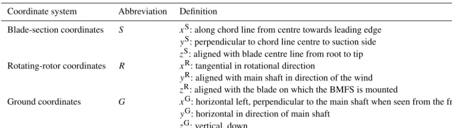
Table 1.Coordinate systems used in this paper.

Coordinate system Abbreviation Definition

Blade-section coordinates S xS: along chord line from centre towards leading edge yS: perpendicular to chord line centre to suction side zS: aligned with blade centre line from root to tip Rotating-rotor coordinates R xR: tangential in rotational direction

yR: aligned with main shaft in direction of the wind zR: aligned with the blade on which the BMFS is mounted

Ground coordinates G xG: horizontal left, perpendicular to the main shaft when seen from the front yG: horizontal in direction of main shaft

zG: vertical, down

2 Method

This section presents the aerodynamic models and the proce-dure used to obtain the free-inflow velocities from a BMFS.

2.1 Coordinate systems

The coordinate systems used in this paper are listed in Ta-ble 1.

Transformation matrices are used to map velocities be-tween the coordinate systems. As an example, the transfor-mation matrix,TRG, describes the rotating-rotor coordinate-system axes in ground coordinates.TRGcan be used to map velocities in rotor coordinates, VR_{, to velocities in ground} coordinates,VG_:

VG=TRGVR. (1)

2.2 Wind speed from a BMFS

The method described in this paper takes as input the effec-tive 3-D inflow velocities measured relaeffec-tive to the blade, lo-cally at the rotor plane, i.e. including the effects caused by the presence of the turbine.

Near the airfoil, the local flow field is deflected and the speed is also influenced by the bound circulation on the sur-face of the airfoil; see the example in Fig. 1. As seen, this effect has a huge impact on the flow velocity measured near the airfoil and must therefore be compensated for before ap-plying the current method. In the current study, however, it is neglected as the two verification environments, HAWC2 and EllipSys3D–Flex5, do not model the surface of the airfoils.

Shen et al. (2006, 2009), Guntur and Sørensen (2014), and Rahimi et al. (2018) present several methods to calcu-late the flow near the airfoil that also take 3-D effects into account, but the methods require information that cannot be obtained directly from a BMFS. Pedersen et al. (2017) de-scribes how to obtain the effective 3-D inflow from the rel-ative wind speed and two perpendicular angles measured by a blade-mounted five-hole pitot, including compensation for bound circulation. The compensation method uses a look-up

9.9 m s1_{, 11}◦

1.8 m s1_{, 91}◦

6.5 m s1_{, 20}◦

15.3 m s1_{, 1}◦

9.3 m s1_{, 2}◦

Figure 1.Near the airfoil, the flow is disturbed by upwash and stag-nation. This effect is not included in the current method.

table generated by 2-D computational fluid dynamic (CFD) simulations, thus neglecting 3-D effects and tip and root vor-tices.

From the relative velocity,Vrel, the wind speed at the rotor plane,Vr, is found by adding the velocity of the sensor,Vs:

Vr=Vrel+Vs. (2)

In this study, the sensor velocity,Vs, includes movement due to rotor rotation and pitch motion. Structural dynamics, e.g. blade deflection, will therefore result in a mismatch between the assumed and the actual sensor velocity.

2.3 Aerodynamic models

therefore expected to be appropriate for the reverse process too.

The aerodynamic models in aeroelastic codes like FAST, Flex5, Bladed and HAWC2 are based on the blade element momentum (BEM) model first presented by Glauert (1935). The original formulation, however, was derived for axis-symmetric, steady and uniform inflow, which is far from the conditions that a real turbine operates in. The BEM model is therefore typically modified and combined with additional sub-models, e.g. for tip loss and for skew and dynamic in-flow. In this study, the aerodynamic model is based on the HAWC2 implementation (Madsen et al., 2018).

2.3.1 Axial induction

When operating, a wind turbine extracts kinetic energy from the wind by reducing the axial wind speed. This reduction is called the axial induction,W_yR; see Fig. 2.

The axial-induced wind speed is defined in terms of the axial induction factor,a:

W_yR=a|V0|, (3)

whereV0is the free-inflow velocity.

For laminated flow through the rotor, the axial induction factor is related to the thrust coefficient,CT, by

CT=4a(1−a), (4)

while empirical results show higher values ofCTfor induc-tion factors above 0.3–0.5 (Eggleston and Stoddard, 1987). The current method uses a third-order polynomial, as de-scribed by Madsen et al. (2018),

a=k3C3T+k2C2T+k1CT, (5)

with coefficientsk3=0.0883, k2=0.0586 andk1=0.2460 that fit to Eq. (4) for lower values of aand to empirical re-sults and actuator disc simulations for higher loading (Mad-sen et al., 2010a).

For an annular ring element at radius r, the thrust coef-ficient is calculated using the formula presented by Madsen et al. (2018):

CT=

V_rel2_xycCy(α)NB 2π r|V0|2

, (6)

whereVrelxy is the relative wind speed in the (xR, yR) plane

(see Fig. 3),cis the chord length,αis the angle of attack,NB is the number of blades and Cy is the projection of the lift

and drag coefficient intoyR:

Cy=cos(φ)CL(α)+sin(φ)CD(α), (7)

whereφ=α+θtwist+θpitchis the angle betweenVrelxyand

the rotor plane.

Figure 2.At the rotor plane, the free-inflow wind velocity,V0, is

reduced by the axial induction,W_yR. A sensor at the rotor plan will therefore measure the reduced velocity,V_r,yR, in the axial direction.

Rotor plane

W

ind

Figure 3.Cross-sectional airfoil element.

From the measurements of a BMFS,Vrelxy andαcan be

obtained directly, and the number of blades, the pitch angle, the radius, the chord length and the blade twist angle are as-sumed to be known. Hence, if the angle-of-attack-dependent lift and drag coefficients are accessible from a look-up table, then the only unknown term on the right-hand side of Eq. (6) isV0.

In aeroelastic simulations,V0 is obtained from the wind input model, but in this case,V0 is the wind speed that we want to find. It can, however, be found using the iterative approach described in Sect. 2.4, such that the induced axial velocity can be calculated via Eqs. (6), (5) and (3).

2.3.2 Tip correction

The relationship between the thrust coefficient and the axial induction factor stated in Eq. (4) is based on the assumption that the induced velocities are constant within an annular el-ement. This is not the case for turbines with a finite number of blades and therefore Prandtl’s tip loss factor, presented by Glauert (1935),

Ftip= 2

πcos

−1

exp

−NB

2

R−r

rsin(φ)

, (8)

factor is straightforward as the only variable on the right-hand side,φ, can be calculated from the BMFS output.

2.3.3 Tangential induction

The tangential induction is a reaction to the torque force and results in a rotation of the wake downstream. The tangential velocity of the wake is defined in terms of the tangential in-duction factor,a0:

W_xR=a0ωr, (9)

whereωis the angular velocity of the rotor.

Variations in the tangential flow due to blade passing can be observed more than one rotor radius upstream. This ef-fect is, however, assumed to be handled by the compensa-tion for defleccompensa-tion and change of flow speed near the airfoil, which is required before the current method is applied (see Sect. 2.2). The current tangential induction model only de-scribes the reaction to the wake rotation that starts near the blades and increases downstream. This effect is assumed to be insignificant upstream. The amount of wake rotation at the position of a BMFS is therefore dependent on the sensor position relative to the blade, the pitch angle and the blade-deflection state. The current implementation of the method assumes full tangential induction, but for some applications, it may be more appropriate to switch it off.

The tangential induction factor is obtained by the formula presented by Madsen et al. (2018):

a0= V 2

relxycCx(α)NB

8π r2_(1−a)|V 0|ω

, (10)

whereCx=sin(φ)CL(α)+cos(φ)CD(α) is the projection of

the lift and drag coefficient intoxR; see Fig. 3.

In Eq. (10), the only unknown term on the right-hand side is alsoV0, which can be found via the iterative approach de-scribed in Sect. 2.4. To help this iterative procedure in finding the right solution, the value ofaused in Eq. (10) is limited to the range[0;0.5].

2.3.4 Radial induction

The radial induction results in an expansion of the flow, as illustrated in Fig. 2. Introducing the radial induction factor,

ar, the radially induced velocity is

W_zR= |V0|ar. (11)

The standard one-dimensional BEM theory does not handle radial induction and therefore the analytical equation derived by Madsen et al. (2010a) is used in the current method:

ar= 1 2.24

CT,avg 4π ln

0.042+ r R+1

2

0.042+ r R−1

2 !

, (12)

whereCT,avgis the average thrust coefficient of the whole ro-tor. In the current model, the revolution-averaged local thrust coefficient of the BMFS is used. This is obviously not the same, and the approximation is therefore only appropriate if the thrust coefficient of the radial position corresponds to the average thrust coefficient of the whole rotor. This is typically not the case near the root and the tip, and even for a sen-sor that is one-third from the tip, some discrepancies must be expected.

2.3.5 Dynamic inflow

The induced velocities are part of an equilibrium which is gradually established between the load on the blades, the rotor wake and the induced velocity at the rotor plane (Sørensen and Madsen, 2006).

Small- and high-frequency turbulence is assumed to pass unaffected though the rotor and can therefore be measured directly, while the effect of large stationary turbulence eddies can be described by the BEM models in Sect. 2.3.1 and 2.3.3. In between, the modification of the wind flow depends on the wake recovery velocity. Snel and Schepers (1995) present different engineering approaches to model the wind turbine response in dynamic inflow.

In the current method, the model used in HAWC2 (Mad-sen et al., 2018) has been implemented with two modifica-tions. This implementation applies two first-order low-pass filters to the induced velocities to model the slow and gradu-ally changing induction,

WR_dyn=0.6LP τNW,WR+0.4LP τFW,WR, (13)

where LP(τ, X) is a first-order low-pass filter. The two filters model the near- and far-wake effects respectively, and their filter characteristics are given by the following.

τNW=τNW∗

1.8R

|V0|min

1−3W

R y,avg

|V0| ,2.0

(14)

τFW=τFW∗

R

|V0|max

1+3W

R y,avg

|V0| ,0.2

, (15)

where

τ_NW∗ = −0.4783(r/R)2+0.1025(r/R)+0.6125, (16)

τ_FW∗ = −0.4751(r/R)2+0.4101(r/R)+1.9210. (17)

Equations (16) and (17) can be calculated straight away, whileV0andWy,Ravgare required for Eqs. (14) and (15).V0 can be estimated as described in Sect. 2.4, while the instant average axial induction of the whole rotor,W_y,R_avg, requires information from the whole rotor, which cannot be obtained from a BMFS.

the filter characteristics may be inaccurate if the induction at the radial position of the BMFS is not representative for the whole blade. The sensitivity to W_y,R_avg is, however, limited and even extreme values have only a minor impact on the final estimated free wind speed.

The other modification is more severe. In HAWC2, the ro-tor is discretized in grid points and the dynamic inflow model is applied to the local induced velocities of each of these grid points. This is possible because the local induction is calcu-lated for each grid point in every time step, and this means that the induction of a certain grid point reflects the current circumstances as well as the history of that particular grid point.

In the current method, only the local induction at the posi-tion of the BMFS is obtainable as no informaposi-tion is available from other parts of the rotor. Applying the dynamic inflow model to the induced velocities at the position of the BMFS means that the estimated induction reflects the history of the moving BMFS instead of a fixed position. In a situation with wind shear, the estimated induction will therefore be too high in the lower part of the rotor and too low in the upper part, resulting in too much variation in the estimated free wind speed.

Instead, the low-pass filters are applied to the induced wind speeds of fixed azimuthal positions. As the BMFS only passes a certain azimuthal position once per revolution, the sample frequencies of these signals are very low and some discrepancies must be expected.

Figure 4 shows the induced velocities in a simulation with turbulent inflow and shear. The quasi-steady induced veloc-ities estimated without the dynamic inflow model, W_yR, are seen to vary much more than the HAWC2 reference, while applying the low-pass filters to the rotating measurements,

W_y,R_dyn, smoothens the induction too much. Applying the low-pass filters to the low-frequency signals of fixed az-imuthal positions,W_y,R_dyn,azi, results in an estimate closer to the HAWC2 reference even though there is still some mis-match.

2.3.6 Skew inflow

In skewed inflow, where the mean wind is not perpendic-ular to the rotor plane due to yaw misalignment, rotor tilt and flow inclination, for example, the axial induction is not directed exactly towards the wind. Hence the speed of the inflow is reduced less, and the thrust is increased. Further-more, variation in the wake vorticity concentration results in an azimuthal-dependent variation in the axial induction; see Fig. 5.

The first effect is modelled by the method described in Madsen et al. (2018) where the axial induction factor is mul-tiplied by a reduction factor,Fa, that is calculated from the

average thrust coefficient,CT,avg, and the skew inflow angle,

100 105 110 115 120

Time [s] 2.8

2.6 2.4 2.2 2.0 1.8

Lo

ca

l in

du

ce

d

ve

loc

ity

[m

s

1]

HAWC2 WR

y (RMS:0.11ms 1)

WR

y, dyn (RMS:0.14ms 1)

W_{y, dyn, azi}R _(RMS:0.05ms 1₎

Figure 4.Local induced axial velocity calculated using HAWC2 and the current method in three configurations:W without the dy-namic inflow model (W_yR), with the dynamic inflow model applied to the rotating measurements (W_y,R_dyn), and with the dynamic in-flow model applied to the low-frequency signals of fixed azimuthal positions (W_y,R_dyn,azi).

Figure 5.Wind turbine in skew inflow. The axial induction varies due to different wake vorticity concentration, and it is not directed exactly towards the wind.

8r.

Fa=k3CT,avg3 +k2CT,avg2 +k1CT,avg+k0, (18)

where

k0=1 (19)

k1= −0.16483r+0.443882r−0.51368r, (20)

k2=0.864683r−2.614582r+2.17358r, (21)

The average thrust coefficient is estimated using the revolution-averaged local thrust coefficient as described in Sect. 2.3.4, and in this case the approximation is also ex-pected to introduce discrepancies. The inflow angle, 8r, which is the angle between the inflow and the rotor axis, i.e. it includes effects of both horizontal and vertical skew inflow, is calculated by

8r=arctan



 q

V₀R_,x2+V₀R_,z2

V₀R_,y 

. (23)

Note that theCT,avg used in Eq. (18) must be limited to the range[0;1]as the model is invalid outside this range.

The azimuthal variation is calculated with a model pre-sented by Madsen et al. (2018). In this model, the axial in-duction factor is multiplied with a rotor-position-dependent factor,Fazi:

Fazi=1−kx

r

Rsin(θrotor)−ky r

Rcos(θrotor), (24)

whereθrotoris the rotor-azimuth position. The factorskxand

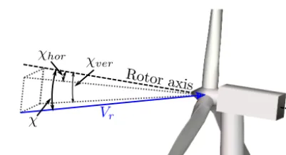
ky depend on the inflow angle in the horizontal and vertical

plane,χhorandχver, respectively; see Fig. 6:

kx=tan(0.4χhor) (25)

ky=tan(0.4χver). (26)

2.3.7 Combining models

The presented aerodynamic models are now combined into a function,fW, that comprises the following steps.

1. CalculateCTusing Eq. (6).

2. Calculate the tip loss factor with Eq. (8).

3. Calculateawith Eq. (5) replacingCTwith_FC_tipT.

4. Apply the skew inflow model by

a. calculating the reduction factorFausing Eq. (18).

b. calculating the azimuthal variation factorFaziusing Eq. (24).

c. applying correction by multiplyinga withFa and

Fazi.

5. Calculate the tangential induction factor using Eq. (10).

6. Calculate the radial induction factor using Eq. (12).

7. Calculate the quasi-steady induced velocities WR=

a0ωr a|V0| |V0|arT.

8. Apply the dynamic inflow model by

a. extracting the induced velocities of each azimuthal position.

Figure 6.χ_horandχverare the angles between the inflow and the

rotor axis in the horizontal and vertical planes respectively.

b. calculating the filter characteristics using Eqs. (14)–(17).

c. applying the dynamic inflow model (Eq. 13) to the induced velocities of each azimuthal position to ob-tainWR_dyn,azi.

Using this function, the estimated induced velocities can be calculated for a givenV0,

West=fW(|V0|). (27)

2.4 EstimatingV0

The flow velocity measured by the BMFS is the sum of the free-flow and the induced velocities, hence

V0=Vr−W. (28)

UsingfW, defined in Sect. 2.3.7, an estimate of the free-flow velocity can be obtained.

V0,est=Vr−fW(|V0|) (29)

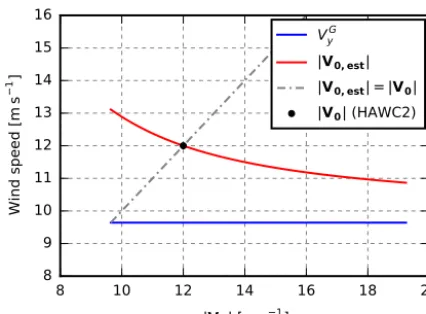
Figure 7 shows the estimated free wind speed, |V0,est|, as a function of|V0|in an example in which the measured wind speed,V_r,yN is around 9.6 m s−1.

We now want to find the correct free wind speed, i.e. the

V0, that, when inserted into Eq. (29), results inV0,estbeing equal toV0 (12 m s−1 in Fig. 7). In other words, we itera-tively solve

|V0| − |(Vr−fW(V0))| =0 (30)

with respect toV0using the Newton–Raphson method and

Vras the initial guess forV0.

2.5 Verification 2.5.1 HAWC2

Figure 7.Example of free wind speed estimation. For|V0| =12,

the estimated free wind speed,|V0,est|, calculated with Eq. (29)

equals|V0|.

has a 6◦ tilt and 3.5◦coning angle and is controlled by the basic DTU Wind Energy controller (Hansen and Henriksen, 2013). The inflow turbulence for the turbulence cases is gen-erated using the Mann model (Mann, 1994).

From the simulations, the relative wind speed is extracted at a point on the blade at radius 36 m, i.e. around one-third from the tip. From this wind speed the estimated free wind speed is calculated and compared to the free wind speed used as the input to HAWC2. Note that the current version of HAWC2 (version 12.5) does not include radial induction, and therefore this model is disabled when testing against HAWC2.

As the current method is based on the same aerodynamic models as HAWC2, one may argue that this verification just adds and subtracts the same value, which obviously results in the original velocity. There are, however, differences that are important to investigate, e.g. the effect of the differences and approximation in the aerodynamic models of the cur-rent method, the effect of a flexible structure and the V0 -estimation procedure.

2.5.2 EllipSys3D–Flex5

The method is furthermore verified using EllipSys3D–Flex5 simulations of a 2.3 MW Siemens turbine with a 93 m ro-tor. In these simulations, the flow field is obtained from LES performed by the finite-volume and incompressible Navier– Stokes solver, EllipSys3D (Michelsen, 1992; Sørensen, 1995). The turbine is modelled using the actuator line method as developed by Sørensen and Shen (2002), in which the in-dividual blades are modelled by imposing body forces into the flow solver. The actuator lines are fully coupled to the aeroelastic tool, Flex5 (Øye, 1996), which models the struc-tural dynamics according to the incoming flow; see Sørensen et al. (2015) for details on the coupling. The inflow

turbu-lence, which is similar to the turbulence of the HAWC2 sim-ulations, is imposed 8.25 radius upstream from the rotor.

From these simulations, the flow speed is extracted at radius 32 m, i.e. also around one-third from the tip. All EllipSys3D–Flex5 simulations use a flexible structural model. Flex5 is based on modal shape functions as opposed to the multibody formulation of HAWC2 and hence does not include torsional rotation of the blades.

To obtain the free-inflow velocities, a separate identical flow simulation is performed, in which the effect of the aero-dynamic forces on the flow is disabled such that the flow is not affected by the turbine. From this simulation the flow field in the vertical plane through the rotor centre is obtained for each time step.

In the aeroelastic HAWC2 simulations, the 3-D correction method by Snel et al. (1993) is applied to the tabulated lift-coefficient polars, while the actuator line simulations have been run without 3-D corrections. The current method re-lies on the same tabulated polars, and additional uncertainty must therefore be expected if the method is applied to fully resolved CFD simulations or real measurements due to dis-crepancies of the tabulated lift and drag coefficients and due to the 3-D effects not taken into account. Furthermore, it should be noted that the two verification environments are not totally independent as both rely on tabulated lift and drag coefficient polars.

2.5.3 Free-flow reference

The estimated free-flow velocities are based on the veloci-ties measured at the sensor position (red dot in Fig. 8). In the current verification, however, the reference free-flow veloc-ity is extracted at the assumed (un-deflected) sensor position (green dot in Fig. 8). This mismatch is expected to introduce some deviation as the turbulence is different at the two posi-tions.

In the HAWC2 simulations, which are based on Taylor’s frozen turbulence hypothesis, the turbulence is transported unaffected by the mean wind, i.e. with constant (free flow) speed along theyGaxis. This means that time can be mapped into space and the free-flow velocities can be extracted from the 3-D turbulence field that is generated prior to the simula-tion.

Figure 8.The estimated free flow at the sensor position (red dot) is compared to the free flow at the assumed position (green dot). In the EllipSys3D–Flex5 simulations, the nearest available free-flow velocity is at the rotor-centre plane (blue dot). The sensor is, how-ever, exposed to “delayed” turbulence structures that originate from a smaller radial position (white dot).

Furthermore, the EllipSys flow is affected by the turbine. Near the rotor, the axial induction reduces the turbulence transport speed, while the radial induction results in an ex-pansion of the flow that moves the turbulence structure out-wards.

This means that the BMFS is exposed to “delayed” turbu-lence structures that originate from a smaller radial position (white dot in Fig. 8), and even more deviation is therefore expected.

3 Results

3.1 HAWC2 verification

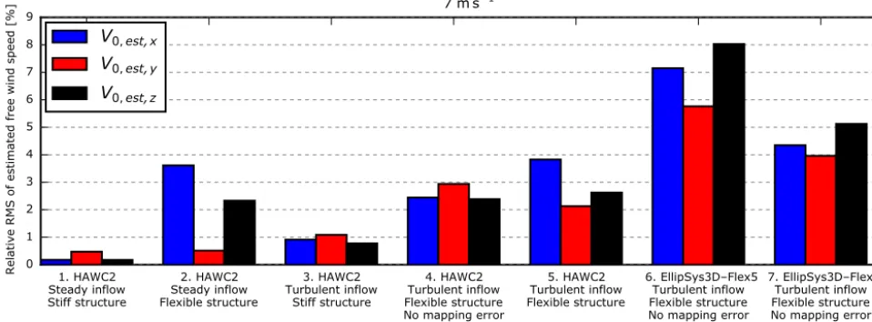
The root-mean-squared error, RMS, of the estimated instan-taneous free wind speed,V0,est, is shown for 7 m s−1in Fig. 9 for HAWC2 simulations of increasing complexity and the EllipSys3D–Flex5 simulations.

Starting with steady, uniform inflow and a stiff structural model, Case 1, the RMS error is very small and the mi-nor deviations between the estimated free velocities and the HAWC2 references in Fig. 10 are caused by the effects of

rotor tilt that are not exactly compensated for by the skew inflow model.

In Case 2, the structural model is flexible. The rotation of the sensor due to the deflection and torsion of the tower and blade results in increased error levels that are clearly seen in thexandzvelocity components in Fig. 10.

The most significant error is the 90◦ phase-shifted sinu-soidal oscillation of the estimated velocities. This error is caused by thrust-dependent flap-wise deflection of the blade that results in a part ofV_r,yR being inaccurately projected onto the zR direction; see Fig. 11. This constant error leads to oscillations of thex andzcomponents in the non-rotating ground coordinate system.

This error is reduced by a counteracting effect, namely the torque pushing the blade forward in the edge-wise direction. At this forward-pushed position, the direction of the actual velocity due to rotor rotation,Vrot∗, is slightly changed, but the blade-section coordinate system is rotated even more as seen in the right-hand side of Fig. 12. A small part ofVrot∗is thereby measured in the radial−zRdirection, while the cur-rent model assumes the rotational velocity,Vrot, to be tangen-tial. This mismatch leads to a torque-dependent error in the −zRdirection that reduces the thrust-dependent contribution from flap-wise deflection.

A closer look at Fig. 10 reveals a positive offset in the es-timatedx component. The reason for this offset, which cor-responds to a spurious side wind, is a combination of two ef-fects, both caused by gravity-induced edge-wise deflections of the blade. When the blades are horizontal, the gravity pulls the blades down towards the earth; see the left- and right-hand sides of Fig. 12. This asymmetric edge-wise deflection leads to a small part ofVrot∗ being measured in the radial −zRdirection on the right-hand side of the rotor and in the +zRdirection on the left-hand side, i.e. in the+xGdirection on both sides. Furthermore, the transition from backward to forward deflection results in the blade moving faster in the upper part of the rotor and vice versa in the lower part. In the current method, however, the assumed rotational speed,Vrot, is uniform. The mismatch results in deviations that also map to+xGin both vertical positions; see Fig. 12.

In combination, these two effects result in the almost con-stant positive offset of theV₀G_,est,xvelocity seen in Fig. 10.

1. HAWC2 Steady inflow Stiff structure

2. HAWC2 Steady inflow Flexible structure

3. HAWC2 Turbulent inflow

Stiff structure

4. HAWC2 Turbulent inflow Flexible structure No mapping error

5. HAWC2 Turbulent inflow Flexible structure

6.EllipSys3D–Flex5 Turbulent inflow Flexible structure No mapping error

7.EllipSys3D–Flex5 Turbulent inflow Flexible structure No mapping error Optimal reference 0

1 2 3 4 5 6 7 8 9

Relative RMS of estimated free wind speed [%]

7 m s 1

V0,est, x

V0,est, y

V0,est, z

Figure 9.Relative RMS of the estimated free wind speed at 7 m s−1. For Cases 4, 6 and 7, “no mapping error” means that deviations introduced in the transformation from the deflected blade-section coordinates to the fixed ground coordinates are not included.

0.4 0.2 0.0 0.2 0.4 0.6 0.8

V

G 0,x

[

m

s

1]

HAWC2 Estimated, stiff Estimated, flexible

6.7 6.8 6.9 7.0 7.1 7.2 7.3

V

G 0,y

[

m

s

1]

0 50 100 150 200 250 300 350 Rotor position [deg]

0.4 0.2 0.0 0.2 0.4 0.6 0.8

V

G 0,z

[

m

s

1]

Figure 10.HAWC2 results including the free wind speed estimated in 13 m s−1steady uniform inflow for stiff (Case 1) and flexible (Case 2) structural models.

Another effect that is seen in higher wind speeds is a neg-ative mean offset in thezcomponent due to tower deflection. In the transformation from rotating-rotor to ground coordi-nates, the angle betweenyRandyGis assumed to equal the tilt angle, but due to tower deflection the real angle is slightly

larger, as it also includes the tower-top deflection angle,θtt; see Fig. 14. A small part ofVris therefore inaccurately pro-jected ontozG, resulting in a small error inV0,est,z.

Figure 11.The rotation angle of the deflected blade section is un-known in the current method. An error is thereby introduced when mapping the measured wind speed,Vr, from the blade-section to

the rotating-rotor coordinates using the transformation matrix,TSR.

The result is a constant error in thezRdirection that leads to sinu-soidal oscillations of thexandzcomponents of the estimated free wind speed seen in Fig. 10.

Figure 12.When the blades are horizontal, a small part ofVrot∗

is measured in the −zR∗ direction on the right-hand side of the rotor and in the +zR∗ direction on the left-hand side due to the gravity-induced deflection of the blade section. Furthermore, the blade moves faster in the upper part of the rotor due to the transition from backward to forward deflection and slower in the lower part. In the current method, however, the rotational speed,Vrot, is assumed

to be tangential and uniform. The mismatch results in a spurious side wind, seen as a mean offset in thexcomponent of Fig. 10.

the transformation from rotating-rotor to ground coordinates. Similarly, the blade deflection and torsion angles can be in-cluded in the transformation from blade-section to rotor co-ordinates. These angles are, however, more challenging to measure due to the large centrifugal force.

In Case 3, a stiff structural model is simulated in turbu-lent inflow. In this case, the estimated free-inflow velocities fall almost on top of the HAWC2 reference despite the dif-ferences in the dynamic inflow model.

Case 4 combines the flexible structure with turbulent in-flow, but the BMFS-measured flow velocities are extracted

Figure 13.The torsion angle of the deflected blade section is un-known in the current method. An error is thereby introduced when mapping the relative velocity,Vrel, from the blade-section to the

ground coordinates using the transformation matrix,T_SG. The re-sult is the overestimation of theycomponent of the estimated free wind speed,V₀G_,est,y.

Figure 14.The tower-top deflection angle,θtt, is unknown in the

current method, and therefore the applied transformation matrix,

TRG, inaccurately projects a small part ofVrontoVr,zG. The result

is the small negative offset in thezcomponent in Fig. 10.

2 1 0 1 2 3

V

G 0,x

[

m

s

1]

HAWC2 Estimated, flexible

4 5 6 7 8 9 10

V

G 0,y

[

m

s

1]

100 110 120 130 140 150 Time [s]

2.0 1.5 1.0 0.5 0.0 0.5 1.0 1.5 2.0

V

G 0,z

[

m

s

1]

Figure 15.HAWC2 results include the free wind speed estimated in turbulent inflow for a flexible structural model (Case 5).

In Case 5, the BMFS-measured flow velocities are ex-tracted in deflected blade-section coordinates and error is in-troduced due to the unknown orientation of this coordinate system; see Figs. 9 and 15. Higher RMS errors are there-fore expected, but in this case, the error of theycomponent is reduced because the error due to coordinate transforma-tion counteracts the error introduced by dynamic deflectransforma-tions. Note that this reduction is highly dependent on the turbine design as it depends on the actual flap and twist properties of the blade, and for other designs the error may be increased instead.

Figure 16 shows the power spectrum density of Case 5. The 1P (once per revolution) oscillating errors seen in thex

andzcomponents in Fig. 10 are seen around 0.2 Hz, while the deviations caused by dynamic deflections are seen in the

y component above 0.4 Hz. At first it seems strange that the energy of theycomponent of the estimated free wind speed is lower than the HAWC2 reference, as the additional veloc-ity due to the movement of the BMFS is expected to increase the energy. In reality, however, the deflection of the structure is correlated with the turbulence, as a blade exposed to a gust will deflect. This means that a BMFS that measures the gust relative to the deflecting blade will measure a less-severe gust with less energy.

Figure 17 shows the instant and revolution-averaged wind direction in a simulation with 20◦ yaw misalignment. The estimated wind direction is seen to follow the HAWC2 refer-ence with a few degrees offset due to the spurious side wind caused by gravity-induced edge-wise blade deflections.

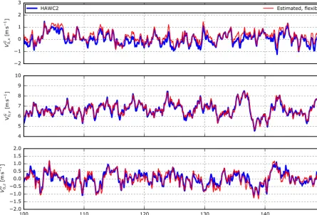
Case 6 is based on the EllipSys3D–Flex5 simulations. The RMS errors are higher than in Case 4, which is the most equivalent HAWC2 case. Note, however, that the numbers are not directly comparable due to the different turbine sizes. The time series are compared in Fig. 18.

For the last case, Case 7, an optimization routine was used to find the optimal reference position with respect to axial and radial offset. For the 7 m s−1the lowest RMS error was found when the estimated free velocities were compared to the free flow that hits the rotor-centre plane 2.2 s before and 4.2 m closer to the rotor centre. As seen in Fig. 9, the error is significantly reduced in all components. It is therefore con-cluded that the relatively high error of Case 6 is more related to the difference between the turbulence at the sensor and the reference position than to deviations introduced in the aero-dynamic models and free-flow estimation procedure.

simu-10 3

10 2

10 1

100

PS

D

(V

G 0,x

)

HAWC2 Estimated

10 3

10 2

10 1

100

PS

D

(V

G 0,y

)

0.0 0.5 1.0 1.5 2.0 2.5 3.0 Frequency [Hz]

10 3

10 2

10 1

100

PS

D

(V

G 0,z

)

Figure 16.HAWC2 results including the power spectrum density of the free wind speed estimated in turbulent inflow for a flexible structural model.

100 110 120 130 140 150 Time [s]

10 15 20 25 30 35 40

Wind direction [deg]

HAWC2

HAWC2, revolution average Estimated

Estimated, revolution average

Figure 17.HAWC2 results including the wind direction derived from estimated free wind speed and HAWC2 reference in a simulation with 20◦yaw misalignment.

lations of the Siemens 3.6 MW turbine. The deviations are mainly introduced in the mapping of velocities from the de-flected blade-section coordinate system to the ground coor-dinate system. The EllipSys3D–Flex5 results are based on

sen-2 1 0 1 2 3

V

G 0,x

[

m

s

1]

EllipSys3D–Flex5 Estimated

4.0 4.5 5.0 5.5 6.0 6.5 7.0 7.5 8.0

V

G 0,y

[

m

s

1]

250 260 270 280 290 300 Time [s]

2.0 1.5 1.0 0.5 0.0 0.5 1.0 1.5 2.0

V

G 0,z

[

m

s

1]

Figure 18.EllipSys3D–Flex5 results including the free wind speed estimated in velocity based on turbulent inflow (7 m s−1) in blade-section coordinates (Case 6).

sor position is different from the free-flow turbulence at the reference position due to expansion, delay and evolvement of the flow. In this case, however, most of these deviations are averaged out, and the error in Fig. 19 is mainly introduced by differences in the induction modelling approach.

The error introduced in the transformation from deflected blade-section coordinates to ground coordinates is clearly seen in all components of the HAWC2 results. In thex com-ponent, the rotor speed and torque-dependent spurious side wind increases the error of the mean wind speed up to rated rotor speed (around 9 m s−1). In they component, the over-estimation due to blade torsion is seen. The error in the mean wind speed in the z direction, due to tower deflec-tion, increases with the thrust up to rated wind speed (around 11 m s−1). Above rated wind speed, the error is rather con-stant as increased drag on the tower counterbalances the de-crease in thrust. Finally, the error, due to flap-wise deflection of the blades, that results in the 1P oscillating deviations of the x and zcomponents is clearly seen in the error of the standard deviation, which peaks with the thrust around rated wind speed.

4 Conclusions

In this paper, a method to estimate the undisturbed free-inflow velocities from the flow velocities measured by a blade-mounted flow sensor, BMFS, has been presented and verified. The method includes a combination of aerodynamic models and procedures to estimate the free-flow velocities from the measurements of a BMFS. The aerodynamic mod-els comprise BEM-based modmod-els for axial and tangential in-duction, a radial induction model and tip loss correction, and models for skew and dynamic inflow. Some of these mod-els require information, e.g. the average thrust coefficient of the whole rotor, that cannot be obtained from a BMFS. In these cases, approximations are used even though they are expected to introduce errors. Most of the models also take as input the free wind speed, which is the final output of the current method. An iterative procedure is therefore used to find the estimated free wind speed.

move-0.1 0.0 0.1 0.2 0.3 0.4 0.5

Er

ro

r

o

f

V

G 0,e

st

,x

[

m

s

1] _{Error of mean (HAWC2)}

Error of mean (EllipSys3D–Flex5)

Error of SD (HAWC2) Error of SD (EllipSys3D–Flex5)

0.1 0.0 0.1 0.2 0.3 0.4 0.5

Er

ro

r

o

f

V

G 0,e

st

,y

[

m

s

1]

4 6 8 10 12 14 16 18 Wind speed [m s 1_]

0.1 0.0 0.1 0.2 0.3 0.4 0.5

Er

ro

r

o

f

V

G 0,e

st

,z

[

m

s

1]

Figure 19.The difference between the mean/SD of the free wind speed at the position of the sensor and the mean/SD of the estimated free wind speed. The HAWC2 results are based on 10 min of simulations of the Siemens 3.6 MW turbine. The deviations are mainly introduced in the mapping of velocities from the deflected blade-section coordinate system to the ground coordinate system. The EllipSys3D–Flex5 results are based on 200 s of simulations of the Siemens 2.3 MW turbine. In this case, the deviations are mainly introduced by differences in the induction modelling approach. Both results are obtained from simulations of a flexible structure in turbulent inflow without shear.

ment of the sensor due to turbulence-induced dynamic de-flections of the structure, and the mismatch between the tur-bulence at the real deflected sensor position and the refer-ence position, i.e. the assumed (un-deflected) sensor position. These effects are highly dependent on the wind speed and the structural design.

Furthermore, the method has been verified by simula-tions performed using EllipSys3D–Flex5: a flexible struc-tural model coupled with a large-eddy simulation (LES) flow solver. In these results, the free velocities estimated using the current method deviate more from the simulated free veloc-ities, but it is concluded that the error is more related to the difference between the turbulence at the sensor and the ref-erence position than to errors introduced in the aerodynamic models and free-flow estimation procedure.

Applied to real measurements, additional uncertainty must be expected due to mounting, calibration and sensor uncer-tainty, discrepancy of the tabulated lift and drag coefficients, and 3-D effects not taken into account.

Appendix A: List of symbols

a Axial induction factor

a0 Tangential induction factor

ar Radial induction factor

c Chord length

CT Trust coefficient

CT,avg Average trust coefficient

Cx Lift and drag coefficient projected intoxR

Cy Lift and drag coefficient projected intoyR

D Aerodynamic drag force

Fa Thrust reduction factor in skew inflow model

Fazi Azimuthal-dependent reduction factor in skew inflow model

Ftip Prandtl’s tip loss factor

fW Function calculating induced velocities

ki,i=0. . .3 Constants

kx,ky Factors in skew inflow model

L Aerodynamic lift force

LP(τ, X) Low-pass filter with filter characteristics,τ

NB Number of blades

r Sensor radius

R Blade tip radius

Tab Transformation matrix from coordinate systemato coordinate systemb

Vr Measured flow velocity at rotor plane

Vrel Measured velocity relative to the sensor

Vrelxy Relative wind speed in the (xR, yR) plane

Vrot Velocity of sensor due to rotor rotation

Vs Velocity of the sensor

V0 Free-flow wind speed

V0,est Estimated free-flow wind speed

W Induced velocity

West Estimated induced velocity

Wavg Average induced velocity

Wdyn Induced velocity, estimated using dynamic inflow model

Wdyn,azi Induced velocity, estimated using dynamic inflow model applied to fixed azimuthal positions

α Angle of attack

χ Angle betweenVrand rotor axis

χhor Horizontal angle betweenVrand rotor axis

χver Vertical angle betweenVrand rotor axis

ω Angular rotor velocity

φ Angle between rotor plane andVrelxy

8r Angle between rotor plane andV0

θpitch Pitch angle

θrotor Rotor azimuthal position

θtt Tower-top deflection angle

θtwist Twist angle

Coordinate systems; see Sect. 2.1

G Ground coordinate system

R Rotating-rotor coordinate system

S Blade-section coordinate system

Modifiers

Competing interests. The authors declare that they have no con-flict of interest.

Acknowledgements. The authors would like to acknowledge Siemens Wind Power for providing data for the simulation model.

Edited by: Luciano Castillo

Reviewed by: Vasilis A. Riziotis and Walter Gutierrez

References

Bak, C., Zahle, F., Bitsche, R., Kim, T., Yde, A., Henriksen, L. C., Hansen, M. H., Blasques, J. P. A. A., Gaunaa, M., and Natara-jan, A.: The DTU 10-MW Reference Wind Turbine, Tech. rep., presented at Danish Wind Power Research 2013, Frederi-cia, Denmark, 27 May 2013, available at: http://www.orbit.dtu. dk (last access: 20 March 2018), 2013.

Barlas, T., van der Veen, G., and van Kuik, G.: Model predictive control for wind turbines with distributed active flaps: incorpo-rating inflow signals and actuator constraints, Wind Energy, 15, 757–771, https://doi.org/10.1002/we.503, 2012.

Brand, A., Dekker, J., de Groot, C., and Späth, M.: Overview of aerodynamic measurements on an Aerpac 25 WPX wind turbine blade at the HAT 25 experimental wind turbie, ECN-DE-Memo-96-014, Energy research Centre of the Netherlands (ECN), Pet-ten, the Netherlands, 1996.

Eggleston, D. M. and Stoddard, F. S.: Wind turbine engineering de-sign, Van Nostrand Reinhold, New York, USA, 1987.

Elliott, D. L. and Cadogan, J. B.: Effects of wind shear and tur-bulence on wind turbine power curves, in: Wind Energy, 10–14, Pacific Northwest Lab., Richland, WA (USA), Presented at the European Community Wind Energy Conference and Exhibition, Madrid, Spain, 10–14 September 1990, available at: http://www. osti.gov/scitech/servlets/purl/6348447 (last access: 20 March 2018), 1990.

Glauert, H.: Airplane Propellers, 169–360, Springer Berlin Hei-delberg, Berlin, HeiHei-delberg, https://doi.org/10.1007/978-3-642-91487-4_3, 1935.

Guntur, S., and Sørensen, N. N.: An evaluation of several methods of determining the local angle of attack on wind turbine blades, J. Phys. Conf. Ser., 555, 12045, https://doi.org/10.1088/1742-6596/555/1/012045, 2014.

Hand, M. M., Simms, D. A., Fingersh, L. J., Jager, D. W., and Cotrell, J. R.: Unsteady aerodynamics experiment phase V: test configuration and available data campaigns, Tech. rep., National Renewable Energy Lab, available at: https://www.nrel.gov/docs/ fy01osti/29491.pdf (last access: 20 March 2018), 2001. Hansen, M. H. and Henriksen, L. C.: Basic DTU Wind Energy

con-troller, Tech. rep., DTU Wind Energy, available at: http://www. orbit.dtu.dk (last access: 20 March 2018), 2013.

Kragh, K. and Hansen, M.: Individual Pitch Control Based on Local and Upstream Inflow Measurements, in: 50th AIAA Aerospace Sciences Meeting including the New Horizons Forum and Aerospace Exposition, Reston, Virigina, Aerospace Sciences Meetings, 9–12 January 2012, American Institute of Aeronautics and Astronautics, https://doi.org/10.2514/6.2012-1021, 2012.

Kragh, K. A., Henriksen, L. C., and Hansen, M. H.: On the Po-tential of Pitch Control for Increased Power Capture and Load Alleviation, in: Torque, the science of making torque from wind, Presented at The Science of Making Torque from Wind 2012, 9– 11 October 2012, Oldenburg, Germany, available at: http://www. orbit.dtu.dk (last access: 20 March 2018), 2012.

Larsen, T. J. and Hansen, A. M.: How 2 HAWC2, the user’s manual, no. December in Denmark. Forskningscenter Risoe. Risoe-R, Technical Report, Risø National Laboratory, Roskilde, Denmark, available at: http://www.orbit.dtu.dk (last access: 20 March 2018), 2007.

Larsen, T. J., Madsen, H. A., and Thomsen, K.: Active load reduc-tion using individual pitch, based on local blade flow measure-ments, Wind Energy, 8, 67–80, https://doi.org/10.1002/we.141, 2005.

Larsen, T. J., Madsen, H. A., Larsen, G. C., and Hansen, K. S.: Val-idation of the dynamic wake meander model for loads and power production in the Egmond aan Zee wind farm, Wind Energy, 16, 605–624, https://doi.org/10.1002/we.1563, 2013.

Madsen, H. A.: Risø-M-2902: Aerodynamics and Structural Dy-namics of a Horizontal Axis WindTurbine – Raw Data Overview, Technical Report Risø-M-2902, Risø National Laboratory, Roskilde, Denmark, 1991.

Madsen, H. A.: Correlation of amplitude modulation to in-flow characteristics, Proceedings of 43rd International Congress on Noise Control Engineering, Inter-noise 2014, Melbournen Australia, 16–19 November 2014, available at: http://www.acoustics.asn.au/conference_proceedings/ INTERNOISE2014/papers/p171.pdf (last access: 20 March 2018), 2014.

Madsen, H. A., Thomsen, K., and Petersen, S. M.: Risø-I-210: Wind Turbine Wake Data from Inflow Measurements using a Five hole Pitot Tube on a NM80 Wind Turbine Rotor in the Tjæreborg Wind Farm, Technical Report Risø-I-2108, Risø National Lab-oratory, Roskilde, Denmark, 2003.

Madsen, H. A., Bak, C., Døssing, M., Mikkelsen, R. F., and Øye, S.: Validation and modification of the Blade Element Momentum theory based on comparisons with actuator disc simulations, Wind Energy, 13, 373–389, https://doi.org/10.1002/we.359, 2010a.

Madsen, H. A., Bak, C., Schmidt Paulsen, U., Gaunaa, M., Fuglsang, P., Romblad, J., Olesen, N. A., Enevoldsen, P., Laursen, J., and Jensen, L.: The DAN-AERO MW Experi-ments: Final report, Denmark. Forskningscenter Risoe. Risoe-R, Danmarks Tekniske Universitet, Risø Nationallaboratoriet for Bæredygtig Energi, available at: http://www.orbit.dtu.dk (last ac-cess: 20 March 2018), 2010b.

Madsen, H. A., Larsen, T. J., Pirrung, G., Verelst, D., and Zahle, F.: An implementation of the BEM model for simulation of non-uniform loading and inflow, in press, 2018.

Mann, J.: The spatial structure of neutral atmospheric surface-layer turbulence, J. Fluid Mech., 273, 141, https://doi.org/10.1017/S0022112094001886, 1994.

Meyer Forsting, A. R., Troldborg, N., Murcia Leon, J. P., Sathe, A., Angelou, N., and Vignaroli, A.: Validation of a CFD model with a synchronized triple-lidar system in the wind turbine induction zone, Wind Energy, 20, 1481–1498, https://doi.org/10.1002/we.2103, 2017.

Michelsen, J. A.: Basis3D – a Platform for Development of Multi-block PDE Solvers, Tech. rep., Danmarks Tekniske Universitet, Kongens Lyngby, Denmark, 1992.

Mikkelsen, T., Mann, J., Courtney, M., and Sjöholm, M.: Wind-scanner: 3-D wind and turbulence measurements from three steerable doppler lidars, IOP Conference Series: Earth and En-vironmental Science, 1, 12018, https://doi.org/10.1088/1755-1315/1/1/012018, 2008.

Mikkelsen, T., Hansen, K. H., Angelou, N., Sjöholm, M., Har-ris, M., Hadley, P., Scullion, R., Ellis, G., and Vives, G.: Li-dar wind speed measurements from a rotating spinner, in: Eu-ropean Wind Energy Conference and Exhibition, available at: http://www.orbit.dtu.dk (last access: 20 March 2018), 2010. Øye, S.: FLEX4 simulation of wind turbine dynamics, in:

Proceed-ings of 28th IEA Meeting of Experts Concerning State of the Art of Aeroelastic Codes for Wind Turbine Calculations. Avail-able through International Energy Agency, 71–76, Danmarks Tekniske Universitet, Lyngby, Denmark, 1996.

Pedersen, M. M., Larsen, T. J., Larsen, G. C., Madsen, H. A., and Troldborg, N.: Turbulent wind field characterization and re-generation based on pitot tube measurements mounted on a wind turbine, in: 33rd Wind Energy Symposium, AIAA SciTech, American Institute of Aeronautics and Astronautics, Kissimmee, Florida, https://doi.org/10.2514/6.2015-1467, 2015.

Pedersen, M. M., Larsen, T. J., Madsen, H. Aa., and Larsen, G. Chr.: Using wind speed from a blade-mounted flow sensor for power and load assessment on modern wind turbines, Wind Energ. Sci., 2, 547–567, https://doi.org/10.5194/wes-2-547-2017, 2017. Petersen, J. T. and Madsen, H. A.: Risø-R-993(EN): Local Inflow

and Dynamics – Measured and Simulated on a Rotating Wind Turbine Blade, Risø National Laboratory, Roskilde, Denmark, 1997.

Rahimi, H., Schepers, G., Shen, W. Z., García, N. R., Schneider, M., Micallef, D., Ferreira, C. S., Jost, E., Klein, L., and Herráez, I.: Evaluation of different methods for determining the angle of at-tack on wind turbine blades with CFD results under axial inflow conditions, Renew. Energ., available online 13 March 2018, in press, 2018.

Schepers, J. G., Brand, A. J., Bruining, A., Hand, M., In-field, D., Madsen, H., Maeda, T., Paynter, J., van Rooij, R., and Shimizu, Y.: Final report of IEA Annex XVIII: enhanced field rotor aerodynamics database, Energy Research Center of the Netherlands, ECN-C-02-016, February, available at: ftp://ftp. ecn.nl/pub/www/library/report/2002/c02016.pdf (last access: 20 March 2018), 2002.

Scholbrock, A. K., Fleming, P. A., Wright, A., Slinger, C., Medley, J., and Harris, M.: Field Test Results from Lidar Measured Yaw Control for Improved Power Capture with the NREL Controls Advanced Research Turbine, in: 33rd Wind Energy Symposium, AIAA SciTech Forum, American Institute of Aeronautics and Astronautics, Reston, Virginia, https://doi.org/10.2514/6.2015-1209, 2015.

Shen, W. Z., Hansen, M. O. L., and Sørensen, J. N.: Determination of Angle of Attack (AOA) for Rotating Blades, available at: http: //www.orbit.dtu.dk (last access: 20 March 2018), 2006. Shen, W. Z., Hansen, M. O. L., and Sørensen, J. N.: Determination

of the angle of attack on rotor blades, Wind Energy, 12, 91–98, https://doi.org/10.1002/we.277, 2009.

Simms, D. A., Hand, M. M., Fingersh, L. J., and Jager, D. W.: Unsteady aerodynamics experiment phases II-IV test configu-rations and available data campaigns, Tech. rep., National Re-newable Energy Lab, available at: https://www.nrel.gov/docs/ fy99osti/25950.pdf (last access: 20 March 2018), 1999. Snel, H. and Schepers, J. G.: Joint investigation of dynamic inflow

effects and implementation of an engineering method, Nether-lands Energy Research Foundation ECN, available at: https: //www.ecn.nl/publications/E/1995/ECN-C--94-107 (last access: 20 March 2018), 1995.

Snel, H., Houwink, R., Bosschers, J., Piers, W., van Bussel, G., and Bruining, A.: Sectional Prediction of 3-D Effects for Stalled Flow on Rotating Blades and Comparison with Measurements, in: Proc. of the European Community Wind Energy Confer-ence, 395–399, Netherlands Energy Research Foundation ECN, Travemünde, Germany, 1993.

Sørensen, J. N., and Shen, W. Z.: Numerical modelling of Wind Turbine Wakes, J. Fluids Eng.-T. ASME, 124, 393–399, https://doi.org/10.1115/1.1471361, 2002.

Sørensen, J. N., Mikkelsen, R. F., Henningson, D. S., Ivanell, S., Sarmast, S., and Andersen, S. J.: Simulation of wind turbine wakes using the actuator line technique, Philos. T. R. Soc. A, 373, 20140071–20140071, https://doi.org/10.1098/rsta.2014.0071, 2015.

Sørensen, N. N.: General Purpose Flow Solver Applied to Flow over Hills, PhD thesis, Technical University of Denmark, available at: http://www.orbit.dtu.dk (last access: 20 March 2018), 1995. Sørensen, N. N., and Aagaard Madsen, H.: Modelling of transient

wind turbine loads during pitch motion, in: Proceedings (on-line) 2006 European Wind Energy Conference and Exhibition, Athens, Greece, 27 February–2 March 2006, vol. 27, 2006. St. Martin, C. M., Lundquist, J. K., Clifton, A., Poulos, G. S., and

Schreck, S. J.: Wind turbine power production and annual en-ergy production depend on atmospheric stability and turbulence, Wind Energ. Sci., 1, 221–236, https://doi.org/10.5194/wes-1-221-2016, 2016.

Taylor, G. I.: The Spectrum of Turbulence, P. Roy. Soc. A-Math. Phy., 164, 476–490, https://doi.org/10.1098/rspa.1938.0032, 1938.

Troldborg, N. and Meyer Forsting, A. R.: A simple model of the wind turbine induction zone derived from numerical simulations, Wind Energy, 20, 2011–2020, https://doi.org/10.1002/we.2137, 2017.