M
M
O
O
D
D
E
E
L
L
I
I
N
N
G
G
N
N
O
O
N
N
L
L
I
I
N
N
E
E
A
A
R
R
D
D
Y
Y
N
N
A
A
M
M
I
I
C
C
A
A
L
L
S
S
Y
Y
S
S
T
T
E
E
M
M
S
S
A
A
.
.
A
A
.
.
A
A
k
k
i
i
n
n
t
t
u
u
n
n
d
d
e
e
11,
,
S
S
.
.
O
O
.
.
N
N
.
.
A
A
g
g
w
w
u
u
e
e
g
g
b
b
o
o
11,
,
O
O
.
.
E
E
.
.
A
A
s
s
i
i
r
r
i
i
b
b
o
o
11,
,
M
M
.
.
A
A
.
.
W
W
a
a
h
h
e
e
e
e
d
d
22,
,
O
O
.
.
M
M
.
.
O
O
l
l
a
a
y
y
i
i
w
w
o
o
l
l
a
a
111
Department of Statistics , Federal University of Agriculture, Abeokuta
2
Department of Mechanical Engineering, Federal University of Agriculture, Abeokuta
Correspondence Author: [email protected]
ABSTRACT: The study of stochastic phenomena has
increased dramatically and intensified research activity in this area has been stimulated by the need to take into account random effects in complicated dynamical systems. Dynamical systems are ubiquitous and are considered to be stochastic processes. In this study, a nonlinear dynamical system was modeled as a solution to an Ito stochastic differential equation
) ( ) ), ( ( )
), ( ( )
(t f x t t t g x t t W t
X
.
where W(t)denotes a Wiener or Brownian motion process while f and gare deterministic functions. The Ito Stochastic Differential Equation was applied to characterize the important functional of the solution process in some intervals
0,t,X
t which satisfies theintegral equation,
t
X
tf
s
X
s
ds
tg
s
X
s
dW
s
X
0 0
,
,
0
. Thesolution of the integral equation is a Lagenvin equation which is an Ornstein-Uhlenbeck (O-U) process
t
tt X dt dW
dX . The O-U process which is a Gaussian process was related to the world of time series analysis. The model was applied to Niger ian monetary exchange rate and compared with the existing models of monetary exchange rate. R package and the Akaike Information Criteria (AIC) were used to provide the model of best fit for the Nigerian monetary exchange rate as an autoregressive moving average of order one which is given to be
S
t
0
.
4287
S
t1
0
.
2099
e
t1
e
t. The results obtained revealed that the structural diffusion model approach gives a first-order autoregressive moving average process in continuous time with differentiation in continuous time corresponding to differencing in discrete time. The derived structural diffusion model has the least AIC value of 1482.61 as compared to the AIC value of 2198.86 from the existing diffusion and normal models.KEYWORDS: Dynamical systems, Stochastic
Differential Equation, Diffusion model, Markov processes.
1. INTRODUCTION
Most real life situations involved modeling of physical processes that evolved with time. The understanding of physical processes that evolved with time is limited by the ability to model a dynamical
system. A dynamical system is a concept in mathematics where a fixed rule describes how a part in a geometrical space depends on time. Dynamical systems are mathematical objects used to model physical phenomena whose state (or instantaneous description) changes over time. These models are used in physics, mathematics, engineering, financial and economic forecasting, environmental modeling, medical diagnosis, industrial equipment diagnosis, and a host of other applications.
can be thought of as an infinite-dimensional vector of random variables. Many practical applications of random sequences involve important case where the underlying statistical property is invariant with respect to time or space. It is often desirable to partially characterize a random sequence based on the knowledge of its first two moment functions which are its mean and variance functions.
The collection of all random functions of a continuous parameter is called a random process. It is important to understand that the basic concept of random process is associated with moment functions. A random process may be uncorrelated, orthogonal and independent of itself and the orthogonally concept is useful only when the random processes under consideration are of zero mean in this case it becomes equivalent to the uncorrelated condition. A random process is also stationary when its statistics do not change with the continuous time parameter. A random process that is particularly useful is a stationary or purely white noise process. Random processes in continuous time can also be defined as processes with independent increment and processes with independent increment are Markov processes. A standard Weiner process is a process with independent increme nt.
Markov processes are random process whose future behavior cannot be accurately predicted from its past behavior and which involves random chance or probability. Markov processes are probabilistic models for describing data with a sequential structure. A Markov process is useful for analyzing dependent random events; that is, events whose likelihood depends on what happened last. Markov processes are continuous time process with a denumerable state space and the theory of Markov processes has developed rapidly in recent years [Dyn06]. A coherent mathematical theory of Markov processes in continuous time was first introduced by Kolmogorov [Dyn06]. Important contributions to this class of stochastic processes were also made by Feller ([Fel67]). More details on Markov Process with denumerable state space can be found in [Chu82] and [KT81].
2. OBJECTIVES OF THE STUDY
The objectives of this study are to study the behavior of nonlinear dynamical system, identify a suitable model structure for the system, estimate the parameters of the identified model and check the adequacy of the fitted model
3. LITERATURES REVIEW
Kalman’s formulation ([Kal60]) of dynamical system makes no assumptions regarding
characteristics (e.g. discrete versus continuous, deterministic versus stochastic of the underlying physical processes. According to [Kal60], a dynamical system is an abstract mathematical object that allows one to talk about physical processes. That is Dynamical systems are mathematical objects used to model physical phenomena whose state (or instantaneous description) changes over time. These models are used in financial and economic forecasting environmental modeling, medical diagnosis, industrial equipment diagnosis, and a host of other applications.
In most dynamical systems which describe processes in engineering, physics and economics, stochastic components and random noise are included. The stochastic aspects of the models are used to capture the uncertainty about the environment in with the system is operating and the structure and parameters of the models of physical processes being studied ([KP92], [SAB12]). Applications of dynamical system are broadly categorized into three main areas which are predictive (also referred to as generative), in which the objective is to predict future states of the system from observations of the past and present states of the systems. The second is diagnostics, in which the objective is to infer what possibly past states of the system might have led to the present state of the system (or observations leading up to the present state), and finally, applications in which the objectives is neither to predict the future nor explain the past but rather to provide a theory for the physical phenomena. These three categories correspond roughly to the need to predict, explain and understand physical phenomena. Predictive and diagnostic reasoning are often described in terms of causes and effects. Prediction is reasoning forward in time from causes to effects while diagnosis is reasoning backward from effects to causes. Not all physical phenomena can be easily predicted or diagnosed. Some phenomena appear to be governed by influences similar to those governing the role of dice or the decay of radioactive material. Other phenomena may be deterministic but the equations governing their behavior are so complicated or so critically dependent on accurate observations of the state that accurate long-term observations are practically impossible.
such functions become stochastic processes in a probabilistic Bayesian framework.
Gaussian processes provide a natural and flexible framework in such circumstances. Nevertheless, the applications of dynamical systems become highly nontrivial when dynamics is nonlinear in the (Gaussian) parameter functions. This happens natura lly for nonlinear systems which are driven by a Gaussian noise process, or when the nonlinearity is needed to provide necessary contrasts (e.g. positively) for the parameter functions
A lot of works had been done on dynamical systems in the last few decades. Some of such works are the work of Mukhin et al ([M+06]) on modified Bayesian approach to the reconstruction of dynamical systems from time series. The work looked at the applicability of Bayesian (statistical) approach to reconstruction of dynamic systems from experimental data. When a dynamical system is known, it is necessary to find values of parameters that determined evolution of the system during time series generation. Such a formulation of the problem arises, for instance, when chaotic regimes of dynamical systems behavior are used for solution of the problem of coded transmission of information (Anishchenko and Pavlov, [AP98]). A formal way of modeling a dynamical system for a necessary positive data is to model the logarithm of the original data. Agwuegbo et al. ([ASA11]) suggested a hierarchical structured model for nonlinear dynamical process while Cai ([Cai12]) proposed a general stochastic differential equation to the transformed variable of dynamical system.
4. METHODOLOGY
In this study, relative change of the process was used as the system evolves with time. The study considered structural model with partial sum as an approach to statistical model building for nonlinear dynamical systems. The approach gave a major method in dealing with drastic quantitative changes in the behavioral pattern of dynamical systems. The dramatic behaviors are associated with some hidden structural changes which we looked at as a function of some characteristic conditions under which the processes occur sometimes called regimes. The structure is based upon the fact that the joint probability distribution of a collection of random variables can be decomposed into series of conditional models and using law of large number with the central limit theorem the combine d distribution follow a normal distribution.
The realization of the stochastic process was partitioned from the view point of partial sums which give rise to a random walk. The series
therefore follow a random walk model which is a martingale. The condition for the random walk is
tj j
t
S
Z
S
1
0 (1)
where and are independent and identically distributed random variables. Recursively, we have the martingale difference given by
t t
t
S
Z
S
1
(2)The generating function is the partial sums
tj j
t
Z
S
1 (3)
In determining the distribution of
S
t,
t
0
,
1
,
2
,...
for a finite t, we made some assumptions about the distribution of
Z
t.
tj j
t
Z
S
1 (4)
If, starting from the initial position,
S
0
0
with thedefining trinomial process given as
0 1 1
t
X (5)
where the probabilities are pfor +1, qfor -1 and r
for 0
In this case, we defined three states for the system and the sequence
X
t is considered as a Guassian random walk, whereX
1,
X
2,...,
X
t are jointly normally distributed.
t
tt
S
dt
dW
dS
(6)If , we have
t t
t
S
dt
dW
dS
(7)Then,
t a t at
S
S
da
dW
S
0 0
0
(8)This is a diffusion process and can be seen as a solution to the stochastic differential equation. The randomness introduced by (8) is an additive noise which makes it equivalent to the Lagenvin equation which is a linear Ito stochastic differential equation. Given that in (7), we get back our random walk model of the form:
t t
t t
t
S
S
W
W
S
1
1
(9)
t
t t
t
S
W
W
S
1
1
1
(10)which can further be written as
(11)
where which is a constant and which is considered to constitute an independent identically distributed sequence of . This gives an autoregressive process of order one. This can be seen to also come from the characteristic of the partial sums combined with the central limit theorem and the martingale difference which can be seen to provide a generalization of an ARIMA
p,d,q
model. The diffusion process in a way transforms the original non stationary series. The Structure introduced into the diffusion process by the partial sums makes the proposed model a more robust model. The structure makes the nonlinear time series stationary and the parameters of the underlying model can easily be estimated. The proposed structural diffusion model was adopted for application in the modeling of the Nigerian monetary exchange rate time series (financial statistics). R software was used in the analysis and parameters estimations of the model. The result from the model was further compared with diffusion, Weiner (which are cons idered as solutions of stochastic differential equation) and ordinary time series model.5. DATA
The empirical data used in this study is the monthly exchange rate of Nigerian Naira to United States Dollar from 1980 to 2013, collected from the website of Central Bank of Nigeria
6. DISCUSSION
The structural diffusion model was used in this study as a limiting distribution of the stochastic differential equation. The study revealed that the AR (1) is a special case of our structural diffusion process. The time plot of the original series (Figure 1) shows an indication that the series is non-stationary and nonlinear. It revealed a dramatic jump in 1999 and high volatility of the monthly exchange rate of Nigerian Naira to United States Dollar.
Nigerian Naira to US Dollar Exchange Rate T ime Plot
Time
E
xch
an
ge
.R
at
e.
ts
1980 1985 1990 1995 2000 2005 2010
0
50
100
150
Figure 1: Time plot of the Exchange rate of Nigerian Naira to US Dollar
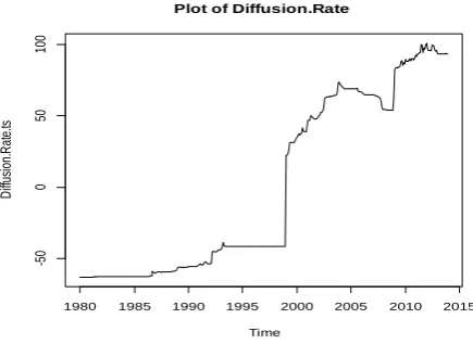
Using the diffusion process, the time plot mimicked the original series as evidenced in Figure 2.
Plot of Diffusion.Rate
Time
D
iff
usi
on
.R
at
e.
ts
1980 1985 1990 1995 2000 2005 2010 2015
-5
0
0
50
100
The time plot of the rate with the Weiner process (Figure 3) also shows that the series is non-stationary and behaves almost similar to the original series.
Plot of Weiner.rate
Time
W
ei
ne
r.r
at
e.
ts
1980 1985 1990 1995 2000 2005 2010 2015
0
1
2
3
4
5
Figure 3: Time plot of the Weiner rate
Figure 4 shows the time plot of the structural diffusion rate. Examining the time plot, it can be seen that the series looks more stationary than what obtains in figures 1, 2 and 3. The dynamics introduced by the structure reduces the nonlinearity of the series.
Plot of Structured Diffusion Rate
Time
S
tru
ct
ur
ed
.D
iff
usi
on
.R
at
e.
ts
1980 1985 1990 1995 2000 2005 2010 2015
-5
0
5
Figure 4: Time plot of the Structured Diffusion rate of Nigerian Naira to US Dollar
The sample autocorrelation function (ACF) and the sample partial autocorrelation function (PACF) are used in the identification of an appropriate time series model. Tables 1 and 2 show the ACF and PACF values for the models of interest. Figures 5 -8 imply the presence of trend in the original, diffusion and Weiner series (as the ACF die of very slowly) while there is no evident trend in the structural diffusion series. The Autocorrelation functions for the structural diffusion series suggest an Autoregressive (AR) or Autoregressive moving average (ARMA) model because of the sinusoidal
behavior of the series. The Partial autocorrelation function (PACF) was further used to verify.
Table 1: Autocorrelation functions at Different Lag values
Lag Value
Normal variable
Diffusion variable
Structured Diffusion
variable
Weiner Variable
0 1.000 1.000 1.000 1.000
1 0.994 0.994 0.569 0.993
2 0.989 0.989 0.236 0.987
3 0.983 0.983 0.051 0.980
4 0.977 0.977 -0.107 0.974
5 0.971 0.971 -0.197 0.967
6 0.964 0.964 -0.293 0.960
7 0.958 0.958 -0.291 0.953
8 0.952 0.952 -0.279 0.946
9 0.946 0.946 -0.234 0.939
10 0.939 0.939 -0.187 0.932
11 0.933 0.933 -0.016 0.925
12 0.926 0.926 0.170 0.918
13 0.920 0.920 0.148 0.911
14 0.913 0.913 0.138 0.904
15 0.906 0.906 0.121 0.896
16 0.899 0.899 0.071 0.889
17 0.892 0.892 -0.001 0.882
18 0.885 0.885 -0.063 0.875
19 0.878 0.878 -0.061 0.868
20 0.871 0.871 -0.105 0.861
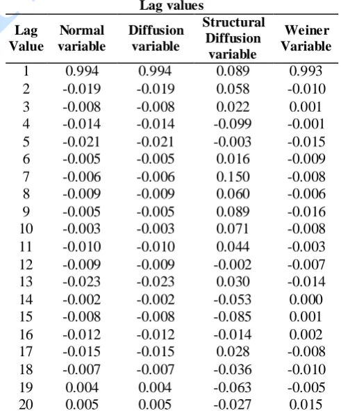
Table 2: Partial Autocorrelation functions at Different Lag values
Lag Value
Normal variable
Diffusion variable
Structural Diffusion
variable
Weiner Variable
1 0.994 0.994 0.089 0.993
2 -0.019 -0.019 0.058 -0.010
3 -0.008 -0.008 0.022 0.001
4 -0.014 -0.014 -0.099 -0.001 5 -0.021 -0.021 -0.003 -0.015 6 -0.005 -0.005 0.016 -0.009 7 -0.006 -0.006 0.150 -0.008 8 -0.009 -0.009 0.060 -0.006 9 -0.005 -0.005 0.089 -0.016 10 -0.003 -0.003 0.071 -0.008 11 -0.010 -0.010 0.044 -0.003 12 -0.009 -0.009 -0.002 -0.007 13 -0.023 -0.023 0.030 -0.014 14 -0.002 -0.002 -0.053 0.000 15 -0.008 -0.008 -0.085 0.001 16 -0.012 -0.012 -0.014 0.002 17 -0.015 -0.015 0.028 -0.008 18 -0.007 -0.007 -0.036 -0.010
19 0.004 0.004 -0.063 -0.005
0 5 10 15 20 25
0
.0
0
.2
0
.4
0
.6
0
.8
1
.0
Lag
A
C
F
ACF Plot for Exchange Rate
Figure 5: Autocovariance function plot of Original Rate
0 5 10 15 20 25
0.
0
0.
2
0.
4
0.
6
0.
8
1.
0
Lag
A
C
F
ACF Plot for Diffusion.Rate
Figure 6: Autocovariance function plot of the Diffusion rate
0 5 10 15 20 25
0.
0
0.
2
0.
4
0.
6
0.
8
1.
0
Lag
A
C
F
ACF Plot for Weiner Rate
Figure 7: Autocovariance function plot of the Weiner Rate
0 5 10 15 20 25
-0
.2
0.
0
0.
2
0.
4
0.
6
0.
8
1.
0
Lag
A
C
F
ACF Plot for Structured.Diffusion.Rate
Figure 8: Autocorrelation function plot (Correlogram) of the Structured Diffusion rate
0.0 0.5 1.0 1.5 2.0
-0
.2
0.
0
0.
2
0.
4
Lag
Pa
rti
al
A
C
F
PACF Plot for Structured.Diffusion.Rate
Figure 9: Partial Autocorrelation function plot of the Structured Diffusion rate
7. MODEL SELECTION AND PARAMETER ESTIMATIONS
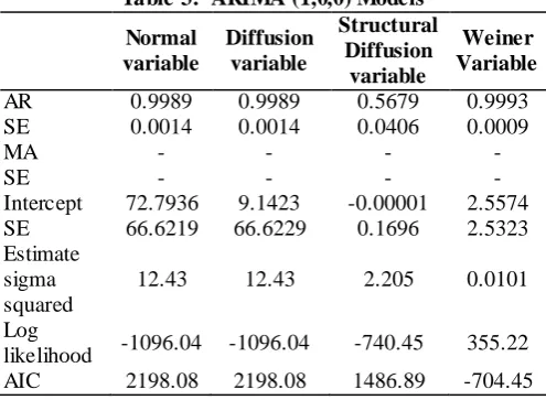
To identify the best fitted model among several linear and nonlinear time series models, the Akaike information criterion (AIC) (Akaike 1974) was use. These criterion measures the deviation of the fitted model from the actual one. The model with the minimum value of AIC was chosen. This work compared twelve different models based on these criteria (Tables 3, 4, and 5).
Table 3: ARIMA (1,0,0) Models Normal
variable
Diffusion variable
Structural Diffusion
variable
Weiner Variable
AR 0.9989 0.9989 0.5679 0.9993 SE 0.0014 0.0014 0.0406 0.0009
MA - - - -
SE - - - -
Intercept 72.7936 9.1423 -0.00001 2.5574 SE 66.6219 66.6229 0.1696 2.5323 Estimate
sigma squared
12.43 12.43 2.205 0.0101
Log
Table 4: ARIMA (1,0,1) Model Normal
variable
Diffusion variable
Structural Diffusion
variable
Weiner Variable
AR 0.9987 0.9987 0.4287 *PCP SE 0.0015 0.0015 0.0769
MA 0.0544 0.0544 0.2099 SE 0.0490 0.0490 0.0839 Intercept 69.8996 6.2484 -0.0001 SE 65.8779 65.8779 0.1542 Estimate
sigma squared
12.39 12.39 2.1710
Log likelihood
-1095.43 -1095.43 -737.30 AIC 2198.86 2198.86 1482.61 *Possible convergence problem
Table 5: ARIMA (1,1,1) Model Normal
variable
Diffusion variable
Structural Diffusion
variable
Weiner Variable
AR 0.9715 0.9715 0.5718 0.0108 SE 0.0993 0.0993 0.0408 1.6776 MA -0.9517 -0.9517 -1.0000 0.0116 SE 0.1348 0.1348 0.0062 1.6888 Estimate
sigma squared
12.34 12.34 2.211 0.0104
Log
likelihood -1088.92 -1088.92 -741.3 342.6 AIC 2183.84 2183.84 1488.59 -679.2
It can be seen clearly that the structural diffusion model has the least AIC values when compared with the other models for all the tentative ARIMA models under consideration. This suggests that the structural diffusion model is better than the other ones under consideration. The Weiner model that seems to have been better than the structural diffusion model has convergence problems in some of its iterations. As a result it cannot be considered adequate for modeling the nonlinear dynamics in the data though very good in modeling linear systems. The selection of a tentative time series model is frequently accomplished by matching estimated autocorrelations with the theoretical autocorrelation ([Agw10]). The ACF and PACF of the structured series indicate stationarity for the series generated from structural diffusion approach.
By fitting ARMA (1,0,1) model, then the fitted Autoregressive Moving Average model is given as:
0
.
1542
0
,
0769
(
0
.
0839
)
2099
.
0
4287
.
0
0001
.
0
t 1 t 1 tt
S
e
e
S
(12)
The numbers in parentheses below the coefficients are standard errors.
8. DIAGNOSTIC CHECKING
The identified model can further be subjected to test in order to examine the quality of the fitted model. This is done by seeing if the residuals form an uncorrelated sequence. The ARMA model diagnostic is shown in figure 10. The first panel of figure 10 shows the standardized residuals from the model fit, second panel shows the ACF for the residual while the third panel shows the p-values for the Ljung-Box statistics. Considering the Ljung-Box Chi-squared statistics, the P-values fall within the allowable limits (upper and lower) which indicates the diagnostic checking for adequacy of the fitted model, the result shows that an autoregressive moving average (ARMA (1,1)) of the structural diffusion model best fit the monetary exchange rate of Nigerian Naira to US Dollar.
The intercept can be considered not significant therefore the model can be narr owed down be
t t t
t
S
e
e
S
0
.
4287
1
0
.
2099
1
(13)CONCLUSION
Diffusion models are under continuous testing. As members of the class of sequential sampling models, they appear to account for experimental data more successfully than any other class of models. This research aims to identify a suitable model for the analysis and forecasting of nonlinear time series analysis. The study constructed a structural stochastic model for the analysis of nonlinear time series using the dynamics of the partial sums and the central limit theorem. Diffusion model was seen as the limiting distribution of the underlying stochastic differential equations. Structural dynamics was further introduced into the resulting diffusion model which gave a better model.
Using the proposed model, the Nigerian exchange rate to US Dollar follows an Autoregressive Moving Average (ARMA (1,1)) model given as:
t t t
t
S
e
e
S
0
.
4287
1
0
.
2099
1
(14)Standardized Residuals
Time
0 100 200 300 400
-6
-2
0
2
4
6
0 5 10 15 20 25
-0
.
2
0
.
2
0
.
6
1
.
0
Lag
A
C
F
ACF of Residuals
2 4 6 8 10
0
.
0
0
.
4
0
.
8
p values for Ljung-Box statistic
lag
p
v
a
lu
e
Figure 10: Residual diagnostics for the structural diffusion series
REFERENCES
[Agw10] S. O. N. Agwuegbo - Hierarchical Model for the Analysis of Large Dimensional State Space; PhD thesis, Department of Statistics, Federal University of Agriculture, Abeokuta , 2010.
[AP98] V. S. Anishchenko, A. N. Pavlon - Global reconstruction in application to multichannel communication, Physical Review E (57) 2455, 1998.
[ASA11] S. O. N. Agwuegbo, A. R. T. Solarin,
O. E. Asiribo - Hierarchical Structured
Model for Nonlinear Dynamical Processes. Journal of the Nigerian
Association of Mathematical Physics 19: 15-20, 2011.
[Cai12] Z. Cai - Econometric Analysis of Financial Market Data. Manuscript for the Department of Mathematics and Statistics, University of North Carolina, Charlotte, U.S.A; 189 pp, 2012.
[Chu83] K. L. Chung - Lectures from Markov processes to Brownian motion, Springer-verlag, New York, 1982. [Cun95] E. P. Cunningham - Digital Filtering:
[Dyn06] E. B. Dynkin - Theory of Markov Processes, Dover Publications Inc. Mineola, New York, 2006.
[Fel67] W. Feller - An Introduction to Probability Theory and its Applications, 3rd ed. Wiley, New York, 1967.
[Kal60] R. E. Kalman - A New Approach to Linear Filtering and Prediction Problems. Journal of Basic Engineering, Transactions ASME, Series D 82: 35-45, 1960.
[KP92] P. E. Kloeden, E. Platen - Numerical Solution of Stochastic Differential Equations. Springer-Verlag Berlin Heidelberg, 1992.
[KT81] S. Karlin, H. Taylo r - A second course in stochastic processes, Academic Press, New York, 1981.
[M+06] D. N. Mukhin, A. M. Feigin, E. M.
Loskutov, Y. I. Molkov - Modified
Bayesian approach for the reconstruction of dynamical system from time series. Physical Review E (73) 036211 (1-7), 2006.
[SAB12] J. A. Shali, J. Akbarfam, H. Bevrani - Approximate solution of the nonlinear stochastic differential equations; International Journal of Mathematical Engineering and Science 1(4): 53-71, 2012.