© Author(s) 2018. This work is distributed under the Creative Commons Attribution 4.0 License.
Dynamic hydrological discharge modelling for coupled climate
model simulations of the last glacial cycle: the MPI-DynamicHD
model version 3.0
Thomas Riddick1, Victor Brovkin1, Stefan Hagemann1,a, and Uwe Mikolajewicz1 1Max Planck Institute for Meteorology, Bundesstraße 53, 20146 Hamburg, Germany
anow at: Institute of Coastal Research, Helmholtz-Zentrum Geesthacht, Max-Planck-Straße 1, 21502 Geesthacht, Germany Correspondence:Thomas Riddick ([email protected])
Received: 16 January 2018 – Discussion started: 29 March 2018
Revised: 3 August 2018 – Accepted: 24 September 2018 – Published: 19 October 2018
Abstract. The continually evolving large ice sheets present in the Northern Hemisphere during the last glacial cycle caused significant changes to river pathways both through directly blocking rivers and through glacial isostatic adjust-ment. Studies have shown these river pathway changes had a significant impact on the ocean circulation through changing the pattern of freshwater discharge into the oceans. A cou-pled Earth system model (ESM) simulation of the last glacial cycle thus requires a hydrological discharge model that uses a set of river pathways that evolve with Earth’s changing orography while being able to reproduce the known present-day river network given the present-present-day orography. Here, we present a method for dynamically modelling river path-ways that meets such requirements by applying predefined corrections to an evolving fine-scale orography (accounting for the changing ice sheets and isostatic rebound) each time the river directions are recalculated. The corrected orography thus produced is then used to create a set of fine-scale river pathways and these are then upscaled to a coarser scale on which an existing present-day hydrological discharge model within the JSBACH land surface model simulates the river flow. Tests show that this procedure reproduces the known present-day river network to a sufficient degree of accuracy and is able to simulate plausible paleo-river networks. It has also been shown this procedure can be run successfully mul-tiple times as part of a transient coupled climate model sim-ulation.
1 Introduction
Results of ocean circulation models are very sensitive to freshwater flux (Maier-Reimer and Mikolajewicz, 1989; Schiller et al., 1997; Stouffer et al., 2006; IPCC, 2013). The accurate modelling of ocean circulation requires the river runoff to be correct for individual ocean basins and dis-tributed with a roughly accurate spatial pattern around each basin’s edge. During the last glacial cycle, the courses of rivers in North America, northern Europe and Siberia were significantly altered by a combination of the physical pres-ence of the ice sheets directly blocking the flow of rivers and the effects of isostatic adjustments altering the orography of ice-free areas (Teller, 1990; Licciardi et al., 1999; Mangerud et al., 2004; Wickert, 2016). Previous studies indicate that modelling of these alterations may play an important role in the success of a transient simulation of the last glacial cy-cle (Alkama et al., 2008; Bahadory and Tarasov, 2018). A comparison of a reconstructed orography for the Last Glacial Maximum (LGM) to a present-day orography indicates that the most significant changes in orography occurred close to the ice sheet. Africa, much of South America and southern Asia were only weakly affected by the changes in the orogra-phy. Here, we introduce a dynamical model of river pathways and hydrological discharge for the simulation of glacial cy-cles that accounts both for the physical presence of ice sheets and for isostatic adjustments.
under-gone further developments since the version (JSBACH 2.0) used for the Coupled Model Intercomparison Project 5 (Tay-lor et al., 2012) as described in Giorgetta et al. (2013). These developments are a new soil carbon model (Goll et al., 2015) and a new five-layer soil hydrology scheme (Hagemann and Stacke, 2015) instead of the previous bucket scheme.
In JSBACH, lateral freshwater fluxes are treated by the Hydrological Discharge (HD) model (Hagemann and Düme-nil, 1998b; Hagemann and Dümenil Gates, 2001). Although the HD model is included in JSBACH, it can also be run independently as a standalone model. In this model, lateral freshwater fluxes are split into three components: base flow, overland flow and river flow. Base flow represents the slow movement of water in the lowest layer of the soil, overland flow represents surface flow outside of channels, and river flow represents channelled surface flow. The HD model is run on a 0.5◦ regular latitude–longitude grid with a daily time step. All three components of the flow from a cell are directed to one of the cell’s eight direct neighbours. Within each grid cell, river flow is modelled through a cascade of linear reservoirs; a cascade of linear reservoirs in each cell is necessary to accurately simulate both the translation char-acteristics (which determine how fast water passes through the cell) and retention characteristics (which determine how much water is stored in the cell) of each cell. The number of reservoirs (nr) is set to 5 (with the exception of cells contain-ing major lakes; however, such lakes are switched off entirely in the version of the HD model used for dynamic hydrolog-ical discharge modelling by this paper as their formulation is unsuitable for modelling lakes that evolve with a chang-ing orography). The river outflow as a function of timeQ(t ) from each reservoir is modelled as
Q(t )=S(t )
k , (1)
whereS(t )is the water content of the reservoir as a function of time andkis the water retention time (also called the re-tention coefficient) of each reservoir. The rere-tention time for riverskris calculated (in days) for each cell in the grid; thus,
kr=0.992 days m−1·1x
s0.1, (2)
where1xis the distance to the centre of the next downstream cell from the centre of the cell under consideration (in me-tres) and defining slope s=1h
1x with1h as the change in orography between this cell and the next downstream cell (in metres). The sign of1his defined such thatsis positive for a downhill slope.sis set to a constant value of 1.315×10⁻⁵ when its original value is either negative or zero. In this pa-per, the set of reservoir retention coefficients for all three of the components of the flow for the whole globe are known collectively as the flow parameters.
In the standard version of the HD model for the present day that is part of JSBACH, the direction of flow is decided by a set of manually corrected present-day river directions
referred to in this paper as the manually corrected (present-day) HD model river directions. These manually corrected (present-day) river directions are derived by first applying a downslope routing to a pit-filled orography; then correct-ing by hand to ensure the correct paths for the world’s major rivers; and finally further correcting by hand the catchments of major rivers based on careful comparison with reference catchments.
The surface runoff and soil drainage of a cell from the JS-BACH model are added to the overland flow and base flow, respectively, and the flow of these through the cell is mod-elled in each case by a single linear reservoir. The water retention time for overland flow reservoirs is calculated us-ing the average slope within a grid box itself when consid-ered on a finer scale (the inner slope) along with the1x as defined above; see Hagemann and Dümenil (1998a) for de-tails. The method for calculating the water retention times for base flow is similar to that given in Hagemann and Dü-menil (1998a) but takes into account some spatial variability (Beate Müller, personal communication, 1998). Base flow re-tention times tend to be roughly 3 orders of magnitude longer than those of overland and river flow. The outflow from all three components is summed and this is used as the input for the river flow of the next downstream cell. When evaluated in an inter-model comparison study (Haddeland et al., 2011), the performance of the HD model as a component of the Max Planck Institute Hydrology Model (MPI-HM) (Stacke and Hagemann, 2012) did not differ significantly from those of similar components of other global hydrology models.
height of riverbeds is overestimated at some points in narrow valleys, thus leading to apparently closed pits or sinks being found in the orography. False sinks also appear at higher res-olutions due to various imperfections in the measurement of orography by satellite (Yamazaki et al., 2017). If river direc-tions are generated from an unmodified orography by the line of steepest descent, then these will be marked as inland sink points, while they are actually unimpeded rivers. Therefore, an algorithm is required to either fill in these false sink points or to let rivers “carve” out of them.
Most previous ESM-based simulations of the last glacial cycle have used the technique of extending present-day river directions to the sea (e.g. Ziemen et al., 2014). This was a suggested method for the Paleoclimate Modelling Intercom-parison Project Phase 3 (PMIP3) (Braconnot et al., 2011, 2012). A number of authors have tackled the problem of modelling river routing during the last glacial cycle. Wick-ert (2016) provides river maps for various time points dur-ing the deglaciation derived directly from a 30 s orography combined with various ice-sheet reconstructions (alongside a useful comparison of these river maps to known data). How-ever, this technique would be too computationally expensive to run fully automatically every 10 years during a transient simulation. Tarasov and Peltier (2006) present a dynamic river routing and lake model for North America during the Younger Dryas that is in many ways similar to that presented here and from which the basic principle of upscaling of ef-fective hydrological heights was taken. However, our new model uses a different combination of upscaling techniques and orography corrections from those of Tarasov and Peltier (2006) as well as a different grid.
Most previous simulations of the last glacial cycle that use coupled global circulation models (GCMs) have only treated time slices; transient simulations have usually been run only in Earth system models of intermediate complexity (EMICs). Goelzer et al. (2012) present a dynamic river routing mod-ule for much of the Northern Hemisphere to produce fresh-water inflows from ice-sheet meltfresh-water (direct precipitation was not considered) for the CLIO ocean model (Goosse and Fichefet, 1999), a component of the LOVECLIM EMIC (Goosse et al., 2010), driven by the ice-sheet model NHISM (Zweck and Huybrechts, 2005). There method is to transform the HYDRO1k hydrologically condition present-day orogra-phy (USGS, 2017) to a 25 km polar stereographic grid by two-dimensional Lagrangian polynomials and use this as a base orography to which to add ice-sheet height corrections and isostatic corrections to during a simulation of the last deglaciation. They note the need to apply some manual cor-rections to resolve blocked valleys in the present-day orogra-phy. The ESM model of Ziemen et al. (2018), which is a pre-cursor to the model the method presented here will be used in, used a simplified method to treat river routing following similar ideas to those presented here.
The first transient synchronously coupled GCM simula-tion of the deglaciasimula-tion was Liu et al. (2009). This used a
time-varying prescribed forcing to simulate the release of glacial meltwater from rivers. However, the PalMod project (Latif et al., 2016), which the approach presented here is in-tended for, aims to run simulations that limit external forc-ings to just solar and volcanic forcforc-ings, thus running tran-sient models using a fully self-consistent ESM and clearly precluding a proscribed-forcing-based approach to meltwa-ter runoff.
An important test of any method is the ability to accurately generate present-day river directions. Large rivers away from the ice-covered regions of Earth do not appear to have drasti-cally changed their course during the last glacial cycle, so for large areas of Earth the river directions should be the same as the present-day river directions for the entire glacial cy-cle. Early testing showed that generating river directions on a 0.5◦grid by simply following the line of steepest descent gives unsatisfactory results for present-day river directions. Using the same technique on a 10 min grid gives better re-sults although there are still some mistakes. Our method aims to correct those mistakes such that the present-day river di-rections can be accurately reproduced on a 0.5◦grid.
2 Method
2.1 Overview of method
The starting point for a simulation of the last glacial cycle is a simulated 10 min resolution orography for timet in the simulation including the height of any ice sheets and isostatic corrections along with the same 10 min resolution orography for the present day; this latter orography is hereinafter re-ferred to as the present-day base orography. From this pair of orographies, the height anomalies for timet with respect to the present can be calculated and applied to a present-day ref-erence orography to which we also apply height corrections (as described below); this is necessary as different present-day orographies can differ markedly due to differences in their methods of fabrication, and thus height corrections must be applied to the particular present-day orography they were created for. (Note it would also be possible to work with a pair of orographies on a different resolution, then remap the anomalies between them to a 10 min resolution.)
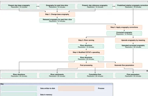
River directions are regenerated every 10 years by a four-step process. A brief outline is given here; detailed descrip-tions of each step are given in the subsequent secdescrip-tions. A flow diagram outlining the steps is given in Fig. 1. Firstly, the orography for timetis adjusted by subtracting the match-ing present-day base orography and addmatch-ing a given reference present-day orography (see Sect. 2.2 and also the discussion in the preceding paragraph). Secondly, a pre-generated set of relative height corrections for a small number of cells (or all cells in the case of North America, where a different algo-rithm is used to generate the corrections) are added to this orography (see Sect. 2.3). These relative height corrections are such that when applied to the given reference present-day orography they return a set of river directions with all of the major errors in river paths and catchments corrected. Thirdly, a set of sinkless river directions on the 10 min grid is gener-ated using the river carving method of Metz et al. (2011) (see Sect. 2.4). Fourthly, these river directions are upscaled to the 0.5◦ grid required by the HD model (see Sect. 2.5). Flow parameters are generated on the 0.5◦grid using an upscaled and sink filled version of the 10 min orography for timet(see Sect. 2.6).
The process described above for the generation of river directions and flow parameters is entirely automatic. Prior to the first application of this process, it was necessary to develop the abovementioned pre-generated set of relative of height corrections. This development was guided and eval-uated by hand although making extensive use of automated tools to expedite the development process and improve the accuracy of the corrections in certain regions. Alongside these automated tools, some corrections were also made by hand. The development of these corrections is discussed ex-tensively in Sect. 2.3.
A useful diagnostic derived from sets of river directions is the total cumulative flow. For each cell, this is the total
num-ber of upstream cells that flow, directly (i.e. without pass-ing through any other cells first) or indirectly (i.e. passpass-ing through other cells first), into that cell. In this paper, we also count the cell itself within the total cumulative flow; thus, the total cumulative flow of any cell is equal to the sum of the total cumulative flows of all cells that directly flow into it plus 1. Total cumulative flow is a property of the river direc-tions as a dry system and does not account for variadirec-tions in rainfall. It also does not account for the variation of latitude– longitude cell surface areas with latitude.
2.2 Changing the present-day base orography
The first step is to change the present-day base orography underlying any given input orography for timetto match the present-day reference orography used to generate the DEM corrections. In the case of all the data generated for this pa-per, this present-day reference orography was ICE-5G ver-sion 1.2 (Peltier, 2004). This is done by applying the follow-ing modification to an input orography on a cell-wise basis: hworking orography=hstandard past orography
−hpresent-day base orography
+hpresent-day reference orography, (3) where hworking orography and hstandard past orography are the height values of a cell at a given time t in a pa-leoclimate simulation, while hpresent-day base orography and hpresent-day reference orographyare the present-day height values of the given cell from two different DEMs. All these oro-graphies will have a 10 min resolution. The present-day base orography is the base orography that is used by a viscoelas-tic Earth model to produce general purpose orographies for times in the past for a wider ESM (in a setup with a coupled ice sheet; otherwise, it is the base orography that was used to derive the ice-sheet reconstruction being used). The stan-dard past orography is then the orography derived from the present-day base orography (again, in a setup with a coupled ice sheet; otherwise, it is just the orography reconstruction being used) for time t via glacial height adjustments from the ice-sheet model and isostatic adjustments from the vis-coelastic Earth model. For any given cell,
hstandard past orography=hpresent-day base orography+hglacier
+1hisostatic, (4)
-Figure 1.Flow diagram illustrating the steps of the method presented here for generating river directions and flow parameters for dynamic hydrological discharge modelling. (Here, “upscale orography by meaning” means simply taking the mean value of the nine 10 min DEM cells contained within the area covered by each 30 min DEM cell as the value of that 30 min DEM cell.)
This first step is necessary because comparisons show due to differing methods of fabrication different 10 min present-day base orographies used in paleoclimate simulations can differ in many cells quite widely (by as much as several hun-dred metres in height in areas of very high inter-cell height variance). These differences are systematic and are appar-ently due to biases in the processing of original satellite data (often on a finer scale) to produce the 10 min present-day orography. In the ESM setups, this method is intended for the present-day base orography will often not be the same as the present-day reference orography, as the present-day base orography is likely to be set for the wider ESM setup the HD model is embedded in, while the present-day refer-ence orography that all the DEM corrections discussed in the next section were generated for is ICE-5G, and it would re-quire significant effort to regenerate these for another refer-ence orography. Preliminary testing showed that the DEM corrections applied in the second step of our method are only valid for orographies generated from the same present-day base orography that the corrections themselves were derived for (i.e. the present-day reference orography), and thus it is
necessary to adjust the input orography such that these cor-rections are still valid.
Although it is intended to use this method with all the input orographies on a 10 min resolution, this step provides the op-tion of alternatively using a paleo-orography and correspond-ing present-day base orography that are of a lower resolution than 10 min.
2.3 DEM corrections
The set of relative height corrections applied in the sec-ond step was derived through comparison with a variety of sources of information on present-day river paths and catch-ments. The development of these relative height corrections was a one-time task which was guided and overseen by hand even when some elements were automated. This set of rela-tive height corrections is provided as input data to each ap-plication of the main river routing and parameter generation process which is in itself fully automatic.
high-resolution orography. Each of these techniques is described (including definitions of the terms “intelligent river burning” and “effective hydrological heights”) individually below. In North America, upscaling effective hydrological heights was used in combination with the other two methods. Only hand application of corrections and intelligent river burning were applied to the rest of the globe. Both combinations of tech-niques are expected to produce satisfactory results; the com-bination of upscaling effective hydrological heights and the other two techniques is expected to produce slightly more ac-curate results in regions where river pathways changed sig-nificantly during the last glacial cycle than just using the other two techniques. However, upscaling effective hydro-logical heights was developed after the other two techniques and it was noted that significant additional effort was re-quired to apply it to North America (justification of this choice of trial region is given below); thus, it was decided not to apply it to the rest of the globe.
The application of both of the first two methods was di-rected by comparison with the manually cordi-rected present-day HD model river directions (through plots of total cumu-lative flow and catchment maps) and by comparing with river directions generated from a finer 1 min orography (through plots of the total cumulative flow only). Differences were resolved using the catchment data of the HydroSHEDS database (Lehner and Grill, 2013). (Online geographical formation from a wide range of sources was used to aid in-terpretation.) The relative corrections applied by hand usu-ally correct the height of the cells of the 10 min present-day orography to the height of the valley floor of the river under consideration observed in the 1 min orography. Occasionally, some guesswork and judgement had to be applied to decide what the true height of the valley floor was; in a few specific cases, the valley was also poorly defined at a 1 min resolution (e.g. the Iron Gates gorge on the Danube).
Intelligent burning of small manually selected regions (usually short sections of an individual river valley) produces similar results but automates the procedure. River directions are generated for the present day from a “super-fine” 1 min orography using the same carving algorithm as described be-low and the total cumulative fbe-low is generated from these super-fine river directions. The 1 min orography is masked outside a selected region and then further masked within that region where the super-fine total cumulative flow is below a given threshold. Then, the height of each cell in the 10 min orography is replaced with the highest unmasked height (if any) within the area of the 1 min orography that corresponds to that 10 min cell (as long as that height is lower than the present height of the cell in the 10 min orography; otherwise, it is left unmodified). This quickly burns a river from the super-fine 1 min orography into the 10 min orography but, unlike regular stream burning techniques (Maidment, 1996; Mizgallewicz and Maidment, 1996; Saunders, 1999), only to the depth observed in a finer orography. Thus, the height of the riverine cells in the burnt area remains realistic to within
the accuracy of a finer orography; thus, the possibility of the river changing direction during the glacial cycle due to changes in the orography remains unimpeded. Note stream burning should not be confused with the largely unrelated technique of river carving. The total cumulative flow thresh-old mentioned can differ for each region where intelligent burning is applied and is set by hand for each case such that only the cells of the super-fine orography through which the main river flows in the region of application in question re-main unmasked. The results of each application of intelligent burning were examined carefully by eye before proceeding. Once the burning process is complete, the changes in the 10 min orography for the present day are converted to rel-ative changes in height (suitable for application at any time during the glacial cycle) by subtracting the original unmodi-fied version of the orography.
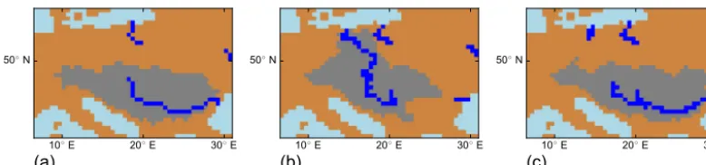
Corrections generated using either one or the other of the first two methods (or a combination of the two) were applied all across the globe to eliminate all significant errors seen in the river directions derived from a 10 min orography, with the exception of some problems related to true sinks which were ignored, as true sinks will not be used when generating dy-namic river directions. Hand application of corrections was usually used where only a few cells needed to be changed; intelligent burning was used where an error in the river di-rections for a particular section of a river needed a larger number of corrections to resolve. Similar results could have been achieved using application of corrections by hand alone but this would have been significantly more time consuming. Figure 2 shows how applying an appropriate correction cor-rects a problem in the catchment of the Danube.
10◦ E 20◦ E 30◦ E 50◦ N
(a)
10◦ E 20◦ E 30◦ E 50◦ N
(b)
10◦ E 20◦ E 30◦ E 50◦ N
(c)
Figure 2.Comparison of the Danube catchment showing the catchment (grey area) and rivers with a total cumulative inflow greater than or equal to 75 cells (blue cells) derived from(a)manually corrected 0.5◦HD model river directions as a reference,(b)automatically generated river directions for a 10 min grid and(c)automatically generated river directions for a 10 min grid once height corrections have been applied to a few selected cells in the orography.
applied beneficially to Eurasia; however, we decided against doing so because of the significant additional effort required. We give here a brief outline of the algorithm; more detailed descriptions of the algorithm are given in Appendices A and B. The algorithm used here works by exploring possi-ble paths through each of a set of sections of a fine orogra-phy that correspond to the individual cells of a coarse orog-raphy. This is performed by flooding each coarse cell on a fine-cell-by-fine-cell basis according to height while filling in any false sinks if necessary. (By the term “flooding”, we mean here processing the cells of the fine DEM in the or-der they would fill with water if the entire coarse cell was to be gradually filled with water starting from the lowest point on the cell’s boundary and assuming the cell was surrounded by a continuous rising body of water such that disconnected basins within the cell could start filling from separate edges.) A path is a pair of cells connected by a particular sequence of intermediary cells, each one of which directly neighbours (including diagonally) the next cell and the previous cell in the sequence. Paths start from the edges of the section (or next to points marked as sea in a land–sea mask) and con-tinue until they meet another edge (or point neighbouring the sea). When a path is finished, it is tested to see if its length exceeds a threshold; this rejects short paths that only cross a single corner of the cell and therefore are not representative of a flow “across” the cell. If it returns back to the edge from which it started, then the greatest perpendicular separation of the path at any point from its starting edge must also ex-ceed a threshold; this rejects paths that flow back to the same edge unless they represent a meander of a significant size. If the path passes these tests, then it is accepted as the low-est valid path through the cell. As any false sinks will have been filled by the algorithm while searching for the path, the last point on the path will be the highest (or joint highest) point on the path. The height of this point is then taken to be the new effective hydrological height of the corresponding coarse cell. Various aspects of the algorithm are illustrated in Fig. 3; these are best understood in conjunction with the two aforementioned appendices.
The parameters MINIMUMPATHTHRESHOLD and MINIMUMSEPARATIONFROMINITIALEDGETHRESHOLD (whose use is described in Appendix A) are both set to 0.5×SCALEFACTOR, where
SCALEFACTOR=
number of latitude points in the coarse grid/
number of latitude points in the fine grid. (5) Originally MINIMUMPATHTHRESHOLD was set to 1.0× SCALEFACTOR to mirror the equivalent parameter in Tarasov and Peltier’s method; however, it was noted that this resulted in narrow channels running near parallel across the border between two cells being “blocked” (both cells hav-ing much higher effective hydrological heights than the rest of the channel and thus causing errors in the river directions generated from the upscaled orography created). The current value prevents these blockages and ensures at least one of the two cells the channel runs through has the same hydrological height as the rest of the channel. The algorithm given here can be used on both hydrologically conditioned orographies such as HYDRO1k (USGS, 2017) (as used by Tarasov and Peltier, 2006) and normal (unconditioned) orographies (with false sinks).
For this paper, we upscale the unconditioned 30 s orogra-phy SRTM30 PLUS (Becker et al., 2009) to a 10 min grid using the effective hydrological height orography upscaling algorithm described above. The orography upscaling process (which need only be run once) takes approximately 25 min to run for the entire globe (from which the section for North America is then extracted) on a single core of a 2015 Mac-Book Pro laptop. This extracted section then forms another component of the set of height corrections once it has been combined with any existing corrections in this region.
Section
Cell Grid
(a)
(b) (c)
(d) (e)
Sea cell
Initially queued cell
Centre cell Skipped neighbour
Neighbour to add to queue Maximum separation from initial edge Route back along path
Figure 3. Diagrams illustrating various aspects of the orography upscaling algorithm. In panel(a), the division of a DEM grid into sections is shown; the upscaling algorithm processes each section separately to produce an effective hydrological height for each sec-tion. Panel(b)shows the initial cells (see main text of Appendix A) added to the queue at the start of the algorithm including the neigh-bours of a sea point. Panel(c)shows three paths: two complete but rejected because they do not meet the selection criteria (see main text) for a valid lowest path, and one incomplete. The short path in the bottom left corner is complete but its length is too short for it to qualify as the lowest valid path through the cell; the longer path on the right is also complete but it returns to the same edge it started at without having met the required maximum separation from the initial edge threshold. The path in the middle, which branches from the short path in the bottom left, is incomplete and a cell at its end is undergoing processing. Half this cell’s neighbours have been added to the queue; the other half have been skipped because they have already been processed. In panel(d), we show a valid lowest path through the cell that returns to its initial edge but meets both of the selection criteria, while in panel(e), we show a valid lowest path through the cell that spans two different edges and has several in-complete paths branching off it.
North American river paths, in some places, the application of this technique introduced new errors. These errors were corrected by a second round of corrections applied by hand. (It was the necessity to verify changes in the river paths after applying effective hydrological heights and make a second
round of additional corrections by hand that required signifi-cant additional effort which, as noted above, in turn drove our decision to limit the application of the upscaling of effective hydrological heights to North America.)
When these corrections are applied to an orography for a time other than the present day, any relative corrections that are beneath ice sheets are temporarily suppressed until the region becomes ice-free once more; thus, the original un-modified height is always used for ice sheets. The corrected orography for a time in the past,t, to which the river carving algorithm is applied in the next section will at a given cell be
hcorrected orography=
(
hworking orography+1hDEM correction, if hglacier=0
hworking orography, otherwise, (6)
where1hDEM correction is the fixed relative DEM correction for the given cell from the set of relative DEM corrections whose development has been discussed extensively in this section;hcorrected orographyis the height of the corrected orog-raphy at the given cell for time t; hworking orography is the height of the intermediary working orography as defined in the previous section; andhglacier is again the vertical thick-ness of the ice sheet in the cell (which is set to zero if the cell does not contain an ice sheet) for timet.
2.4 False sink removal
cell and then added to the queue themselves unless they have already had directions assigned to them previously (in which case they are ignored as they were processed previously; the river direction assigned to them is unchanged and they are not added to the queue again). By following this procedure when the lowest point on the lip of a sink is reached, the al-gorithm will follow the river down to the bottom of the sink marking a river path that carves out of the sink (i.e. flows up-hill) from the bottom to the lip of the sink. Within the sink, cells not directly neighbouring the exit path will drain to-wards the bottom of the sink where they will join the exit path. The possibility exists to mark some points as potential true sinks (i.e. real endorheic basins); if these are in a sink, then they are treated as the outflow point for that sink; other-wise, processing continues normally. However, this option is not used as it has been decided to remove all true sinks com-pletely when generating dynamic river directions. This closes the water balance using the assumption that precipitation in an endorheic basin would eventually end up in a neighbour-ing non-endorheic basin either through atmospheric recircu-lation or via a slow seepage of ground water. This assumption is made in the absence of a full model of dynamic lakes; it may be removed if these are treated by further work. In this absence of dynamic lakes, it is necessary to make this as-sumption (or a similar asas-sumption that the water flowing to true sinks can be redistributed directly into the ocean) as wa-ter conservation is critical for multi-millennial transient pa-leoclimate simulations. The effects of omitting true sinks are effectively the effects of not modelling dynamic lakes; these effects are discussed in Sect. 6.1. It is still useful to include true sinks when generating data for validation against known modern-day river direction information (which also includes true sinks).
2.5 Upscaling procedure
The fourth step upscales the 10 min river directions that have been generated to a 0.5◦grid using a variant of the Cell Outlet Tracing with an Area Threshold (COTAT)+ upscaling algo-rithm (Paz et al., 2006). This algoalgo-rithm itself contains three major steps. The grid cells of the finer grid, referred to as pixels, are grouped into sections corresponding to the cells of the coarse grid (these sections are then themselves referred to as cells). The first step is to identify the outlet pixel of each coarse grid cell. This is the pixel with the highest cumula-tive outflow which meets at least one of two criteria. The first criterion is that the path leading to the pixel through the cell (along the line of greatest overall cumulative flow) sat-isfies a minimum path length threshold. The second criterion is that the pixel drains the largest number of pixels within the cell in question. These are introduced so that the river direction of the cell is determined by the main river flowing through the cell excluding any rivers that just skirt through a corner of the cell unless they have a tributary which drains a large fraction of the cell itself. The second step is to decide
a flow direction for each cell. For each cell, the flow path is traced downstream from the chosen outlet pixel until its to-tal cumulative flow has increased by a set amount or it exits from the direct neighbours of the central cell. The river di-rection points towards the cell where the downstream tracing finishes. This increases the use of diagonal river directions compared to simply choosing the cell that the outlet pixel di-rectly flows into. The third step is to remove the rare situation of crossing river directions by redirecting the flow direction of the cell whose outlet pixel has the lower total cumulative flow into the same cell as the cell whose outlet pixel has the higher total cumulative flow flows into. However, this third step is not used in the variant of the algorithm used here. Al-though rivers crossing is clearly unphysical if it did occur, it would not negatively affect the quality of the upscaling in terms of the mapping of catchments to river mouths. Instead, two scans are run to identify rarely occurring loops in the up-scaled flow directions and reprocess the cells where they are occurring to remove them; in each case, favouring preserving the river with the highest total cumulative flow.
2.6 Flow parameters
at an oblique angle to the grid and thus varies with time); oth-erwise, they are generated by a similar technique to the river flow retention coefficients using data from timetonly. Base flow retention coefficients use a similar approach, using ex-isting data for the present day where available to account for spatial variability otherwise reverting to the original formu-lation of Hagemann and Dümenil (1998a). This approach to overland flow and base flow retention coefficients is chosen for simplicity; accurate representation of temporal changes in these parameters is not considered to be important provided plausible values are used throughout the transient simulation. The initial reservoirs for starting a transient paleoclimate simulation are set by adapting the present-day initial reser-voirs from the existing HD model. Using a set of present-day river directions and flow parameters generated by the method presented in this paper, points that are ocean due to land–sea mask differences (possible as present-day land–sea masks can vary), lakes, negative flows (possible due to P−E on glaciers) and wetlands are all removed and replaced with the value(s) of the highest (non-removed) direct neighbour or if that is not possible then the global average(s) (for that/each reservoir type). This setup was run for a year for the present day. It is observed that the model reaches equilibrium or very close to equilibrium after running half a year when no lakes or wetlands are included. The restart file from this run pro-vides starting values for transient paleoclimate simulations using dynamical hydrological discharge after performing the same set of operations as above on it again (though obviously there are no lakes or wetlands to remove) using the river directions and flow parameters generated from the starting orography and land–sea mask of the transient climate simu-lation. The initial reservoirs for periodic restarts of a transient paleoclimate simulation (that occur after stopping to recalcu-late river directions and flow parameters and any other slow processes necessary) are taken from the restart file produced at the end of the previous run segment. If changes in the land– sea mask have created new land, then all of the reservoirs in the new land cells are initialised to zero, while if changes in the land–sea mask have flooded land, then the contents of all of the reservoirs in the flooded land cells are released into the ocean.
2.7 Code and performance
Both the sink filling and river carving algorithms and the orography upscaling algorithm are written in (object-oriented) C++ and share a single code base. The river catch-ments on the 10 min scale used in figures are also generated simultaneously to river carving by the same code. This is effectively an application of the algorithm of Beucher and Meyer (1992) and Beucher and Beucher (2011). The CO-TAT+ variant used is written in object-oriented Fortran 2003. Other ancillary tasks are performed in Fortran 90 or Python. Both the sink filling/river carving/orography upscaling algo-rithms and the COTAT+ river direction upscaling algorithm
are designed to be easily extendable to other grids (such as the triangular grid of the ICON-ESM; Zängl et al., 2015). The total runtime of the code required to generate river di-rections and flow parameters for a given time slice on a mod-ern desktop PC with a (multi-core) 3.5 GHz Intel processor is about 1 min. It is clear from these results that the per-formance of this code presents no significant issues and it will clearly not impede the performance of the coupled cli-mate model simulations in which it is intended to be embed-ded. Given the short runtime of the code, parallelisation was deemed unnecessary.
3 Evaluation for the present day
River directions were evaluated using the total cumulative flow and river catchments. An evaluation of the areas of catchments of major rivers derived from the river directions generated from a 10 min orography using the method pre-sented here shows that in most cases they match those of the manually corrected river directions currently used in JS-BACH to within 5 %. Evaluation by eye confirms that the catchment shapes are also very similar. All significant dis-agreements were identified as being due to minor deficien-cies in the manually corrected JSBACH river directions by cross checking against the HydroBASINS catchments. Hy-droBASINS are a part of the HydroSHEDS dataset (Lehner and Grill, 2013). Adjustments were made to discount dis-crepancies due to uncorrected true sinks in the river direc-tions derived from the 10 min orography (as noted above, some true sink related errors were ignored in the creation of the corrected orography as all true sinks will be removed for actual paleoclimate simulations). Figure 4 shows zoomed sections comparing the catchments of three major rivers cho-sen as examples for the manually corrected 0.5◦present-day HD model river directions and for those derived from the 10 min river directions generated from a corrected 10 min present-day orography. While good agreement is generally observed in these three examples, a number of differences are clear around the edges of the catchments. Each differ-ence comprising more than one or two cells has been checked against various sources of hydrological information; in every case, the difference is either due to a minor error in the man-ually corrected JSBACH river directions or lies in an area of desert with no discernible rivers.
30◦ E 40◦ E 30◦ N
20◦ N
10◦ N
0◦
Nile
110◦ W 100◦ W 90◦ W 80◦ W 50◦ N
40◦ N
30◦ N
Mississippi 100◦ E 110◦ E
30◦ N
20◦ N
10◦ N
Mekong
Sea Land
Default HD catchment Common catchment Dynamic HD catchment
Figure 4. Comparison of the manually corrected 0.5◦ catchments for the present day (“default HD”) to those of the 10 min directions generated from a corrected 10 min present-day orography (“dynamic HD”) for the Nile, Mekong and Mississippi.
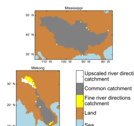
true sinks, then these problems disappear. The only signifi-cant problem is the upper reaches of the Mekong catchment being incorrectly directed into the Yangtze, while some wa-ter from the Salween River is diverted into the Mekong (thus, overall, the total area of the Mekong catchment is roughly correct but the Salween catchment’s total area is too small and the Yangtze’s too great, and the actual location of all three rivers’ catchments is partially incorrect). This is illus-trated in Fig. 5. This problem is due to the COTAT+ algo-rithm being unable to cope with the three rivers flowing very close to each other in Yunnan province, China. This could be fixed by allowing non-local flows and using an algorithm like the FLOW algorithm (Yamazaki et al., 2009) but this would require considerable modification of the existing JS-BACH HD model. Another possibility would be to run both COTAT+ and an algorithm that generates non-local flows and use the latter to identify and remove disconnects in the for-mer by slightly displacing river paths where necessary.
Figure 6 shows a validation of the automatically gener-ated and upscaled river directions against the manually cor-rected river directions. Although many differences are ob-served, most of these do not affect which outlet drains which area. Differences that result in a significant change in outlet position for a significant area (more than a couple of cells) have been checked against various sources of hydrological information (primarily HydroBASINS); in all cases, they are either due to minor errors in the manually corrected JSBACH river directions or lie in areas of desert with no discernible rivers (with the exception of differences connected to the
110◦ W 100◦ W 90◦ W 80◦ W
50◦ N
40◦ N
30◦ N
Mississippi
90◦ E 100◦ E 110◦ E
30◦ N
20◦ N
10◦ N
Mekong
Sea Land
Fine river directions catchment
Common catchment Upscaled river directions catchment
Figure 5.Comparison of the upscaled catchments of the Mississippi and Mekong on a 0.5◦grid to the original 10 min version.
Mekong for which the automatically generated and upscaled river directions are erroneous due to a deficiency of the up-scaling procedure as previously discussed).
180◦ 120◦ W 60◦ W 0◦ 60◦ E 120◦ E 180◦ 90◦ N
60◦ N
30◦ N
0◦
30◦ S
60◦ S Sea
Minor catchments Dynamic HD river path Discrepancy in catchments Common catchment Glacier
Figure 6.Comparison of the most significant present-day river catchments derived using the method presented here (“dynamic HD”) to the manually corrected HD model river directions. Discrepancies are shown in red; areas of catchments that are common between both models are marked in grey. The three different shades of grey are used to pick out individual river catchments; no significance is attached to the shade chosen for each river. Dynamic HD river paths (defined as cells with a cumulative flow of 100 cells or more) are marked to aid orientation.
points) were compared to the those currently in JSBACH by running the model for 1 year in a standalone setup with rainfall data as a forcing and comparing the total daily dis-charge into the ocean (including inland sinks in the case of the current model). The results (not shown) show a very close match; the small discrepancies observed are expected as the current JSBACH model includes inland sinks, lakes and wet-lands, all excluded in the dynamic HD model presented here. The present-day river directions and flow parameters gen-erated using the method presented in this paper have been applied in a pre-industrial-control simulation using the cur-rent coarse-resolution (CR) version of MPI-ESM. The sim-ulation was started from a steady-state simsim-ulation obtained after a long (more than 6000-year) spin-up with the man-ually corrected present-day HD model river directions and flow parameters. The results (not shown) indicate only small local changes, especially in surface salinity close to river mouths. The only exception to this was that the total water flux into the Indo-Pacific was increased and the total wa-ter flux into the Atlantic was reduced when using dynamic river directions. The reason for this is that the flow into in-land sinks in Asia that was spread evenly around the world’s river mouths when using manually corrected HD river direc-tions was now added to rivers flowing into the Indo-Pacific (as inland sinks had been removed). The large-scale circula-tion remained largely unchanged.
4 Application to an LGM simulation
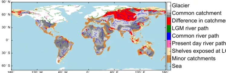
Figure 7 shows a comparison of the 0.5◦ river directions derived by the dynamic HD method presented here using the present-day ICE-6G_C orography and the reconstructed LGM ICE-6G_C orography (Argus et al., 2014; Peltier et al., 2015). The main differences from the present day that are observed in North America at the LGM are an expansion of the catchment of the Mississippi to drain a significant area of the ice sheet surface into the Gulf of Mexico and an
ex-pansion of the Yukon to drain part of the northwestern ice sheet surface into the Pacific Basin. In Eurasia, the flow of a large number of rivers in western Siberia and Scandinavia is blocked by the Fennoscandian ice sheet at the LGM. This forces these rivers to flow either west or east along the ice-sheet edge (and thus merge to form two very large rivers). To the west, this continues until the flow pathway reaches the North Atlantic Ocean at the western end of the ice sheet; to the east, the flow pathway eventually makes a short de-tour south before reaching the Arctic Ocean just beyond the eastern end of the ice sheet. Elsewhere on the globe, at the LGM, rivers simply extend from their present-day mouths to the new extended LGM shoreline.
To validate our approach, we compared river directions generated with our method for the LGM to river directions generated directly from a fabricated LGM orography on a 30 s grid created by adding the difference between the re-constructed LGM ICE-6G_C orography and the present-day ICE-6G_C orography to the present-day SRTM30 PLUS orography. Here, we used the ICE-6G_C orographies on a 10 min grid; we converted the difference between them to a 30 s grid to match that of the SRTM30 PLUS orography by assigning each 30 s cell the value of the 10 min cell it would lie within were the 10 min grid overlaid on the 30 s grid. (This resulted in a blocky structure to the resultant fabricated orog-raphy.) We then applied the river carving algorithm as de-scribed in Sect. 2.4 directly to the fabricated 30 s orography and compared the catchments of the rivers produced to those produced by applying our method to the reconstructed LGM ICE-6G_C orography.
180◦ 120◦ W 60◦ W 0◦ 60◦ E 120◦ E 180◦ 90◦ N
60◦ N
30◦ N
0◦
30◦ S
60◦ S Sea
Minor catchments Shelves exposed at LGM Present day river path Common river path LGM river path
Difference in catchments Common catchment Glacier
Figure 7.Comparison of the most significant rivers at the LGM and present day generated by the method described in this paper using the ICE-6G_C reconstructed orography for the LGM. Rivers are shown where the cumulative flow to a given grid cell (on the HD grid) is greater than or equal to 100 cells. The various colours show various rivers that existed only at the LGM (green), only at the present day (pink) or at both (blue). The catchments of major rivers are marked. Differences between the catchments are shown in red; areas of catchments that are common between both time slices are marked in grey. The three different shades of grey are used to pick out individual river catchments; no significance is attached to the shade chosen for each river. Continental shelves which were exposed as dry land at the LGM by the significantly lower sea level are also marked. Rivers shown on the surface of ice sheets are topographically defined rivers, and thus their presence does not necessarily imply that there were rivers running off the northern slopes of the Laurentide and Fennoscandian ice sheets.
fabricated orography. Investigation shows this is because fine detail of narrow valleys not present in the present-day ICE-6G_C orography or the reconstructed LGM ICE-ICE-6G_C orog-raphy is “printed” from the SRTM30 PLUS orogorog-raphy onto the surface of the ice sheet by the fabrication process used; this fine detail allows a river to flow into a catchment to the north following a river pathway in the underlying orography rather than west into the Yukon as it does in the river di-rections generated using our dynamic HD method. Given the considerable thickness of the ice sheet at this point, it is likely this would not occur physically but the detail of the underly-ing orography would be smoothed over by the ice sheet.
To test the effect of dynamically modelling river directions at the LGM against the approach typically used in climate model simulations of this time slice of simply extending the present-day rivers to the new shoreline, two simulations were performed using the boundary conditions from the MPI-ESM LGM simulation of Klockmann et al. (2016). Both simula-tions integrated the same model as for the present-day ex-periments discussed above using the restart files from Klock-mann et al. (2016), but the river direction file differed be-tween the two simulations. One used dynamic river direc-tions generated as described in this paper using the ICE-6G_C orography reconstruction; the other simply extended the present-day river directions (including inland sink points) used in JSBACH as standard to the new coastlines. This is consistent with the PMIP3 approach (Braconnot et al., 2011, 2012) for coupled LGM simulations.
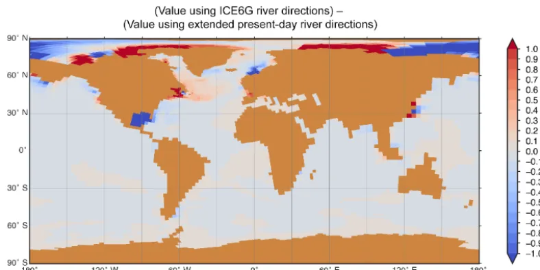
Analysis of the two runs is based on climatologies of the last 500 years. Figure 8 shows the difference in freshwater flux into the ocean between the two simulations (including both river outflow andP−Eover the ocean surface) on the ocean grid. Figure 9 shows the total freshwater flux into the Indo-Pacific and Atlantic basins as an integrated total from
the North Pole to each specific latitude (the implied south-ward ocean freshwater transport). In both basins, a number of localised dipoles are observed; these represent minor dif-ferences in the position of the mouth of major rivers and will have very little effect on global circulation patterns. The overall freshwater influx into the Atlantic is reduced and the overall freshwater flux into the Indo-Pacific increased when using dynamic river directions; this change is likely at least partially due to the removal of inland sink points. A signif-icant increase in the catchment of the Mississippi (and thus its outflow) occurs with dynamic river directions, while to the north the St. Lawrence ceases to exist (although a sig-nificant amount of water continues to drain off the ice sheet in this area); thus, there is an overall movement of freshwater southwards. As expected, the Fennoscandian ice sheet causes a significant lateral movement of water to its ends when us-ing dynamic river directions. In the Pacific, the main change observed is the merging of the Yangtze and Yellow rivers at their mouths when using dynamic river directions; this pro-duces a large peak in the river outflow but this peak is off-set by two troughs on either side. With dynamic river direc-tions, the outflow from the Yukon is significantly increased and water is diverted from the North American Arctic coast to the northern Pacific coast of North America. In the Indian and southern Pacific basins, little overall change is observed, though there are several large local dipoles.
Figure 8.Changes in the freshwater flux into the ocean between simulations run in the MPI-ESM model of the LGM using extended present-day river directions and using dynamic river directions. The changes are defined such that an increase in the version using dynamic river directions is positive. A symmetrical logarithmic colour scale is used: above 1, the colour scale is logarithmic; between 1 and−1, the colour scale is linear; below−1, the colour scales according to the negation of the logarithm of the change’s magnitude.
the atmospheric temperature. An increase in the sea surface temperature (SST) of almost 1◦C is observed in the subpolar
northwest Atlantic. In the Norwegian Sea and the Irminger Sea, salinity is reduced when using dynamic river directions. The enhanced stability then reduces convection and the up-ward mixing of heat in the ocean to the surface. The con-sequences are a reduction in the SST by about 1◦C and
en-hanced sea ice cover.
These changes in freshwater flux forcing have also conse-quences for the ocean circulation. In the northwest Atlantic, the subtropical gyre expands northward in the western half of the basin and the subpolar gyre becomes weaker and con-tracts when using dynamic river directions. However, these changes have only a negligible effect on the Atlantic merid-ional overturning circulation.
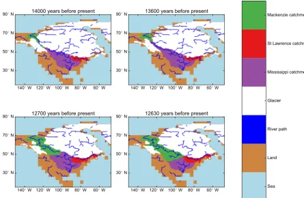
5 Application to a selected sequences of times during deglaciation
As a demonstration of the modelling of the dynamic evolu-tion of river pathways in North America by the technique presented here, we show in Fig. 11 the major rivers and the most important catchments as generated by the technique for a sequence of four times selected from the last deglaciation . The ice-sheet height and isostatic adjustments are taken from ICE-6G_C, while the land–sea mask is generated using the technique given in Meccia and Mikolajewicz (2018).
6 Discussion and conclusions 6.1 Limitations
interac-600 000 400 000 200 000 0 200 000 400 000 600 000 Implied southward ocean freshwater transport (
m
3s
−1)90 S◦ 60 S◦ 30 S◦ 0 ◦ 30 N◦ 60 N◦ 90 N◦
Latitude
(a)
Atlantic
Extended present-day river directions ICE6G river directions
600 000 400 000 200 000 0 200 000 400 000 600 000 Implied southward ocean freshwater transport (
m
3s
−1)90 S◦ 60 S◦ 30 S◦ 0 ◦ 30 N◦ 60 N◦ 90 N◦
Latitude
(b)
Indo-Pacific
Extended present-day river directions ICE6G river directions
40 000 20 000 0 20 000 40 000 60 000
Change in implied southward ocean freshwater transport (
m
3s
−1) 90 S◦60 S◦ 30 S◦ 0 ◦ 30 N◦ 60 N◦ 90 N◦
Latitude
(c)
(
Value using ICE6G river directions)
−(
Value using extended present-day river directions)
Atlantic Indo-Pacific
Figure 9.Comparison of the implied southward ocean freshwater transport between simulations run in the MPI-ESM model of the LGM using extended present-day river directions and using dynamic river directions for(a)the Atlantic Ocean and(b)the Indo-Pacific. Plot (c)gives the difference between the two simulations for both basins. The freshwater transport is defined such that a net addition of freshwater to the ocean (via precipitation and river discharge) is positive and a net removal of freshwater (via evaporation) is negative.
tions (Hostetler et al., 2000; Krinner et al., 2004) and pre-cludes both the inclusion of the mass of the water in the lakes as a feedback to the viscoelastic Earth model and the mod-elling of lacustrine calving of ice sheets where they are in direct contact with an adjacent lake.
be-Figure 10.Changes in the surface ocean salinity between simulations run in the MPI-ESM model of the LGM using extended present-day river directions and using dynamic river directions. The changes are defined such that an increase in the version using dynamic river directions is positive.
tween the current sill height and previous higher sill heights may have had a deciding effect on which outlet overflowed in earlier phases of the lake’s development. Wickert (2016) argues that in the case of Lake Agassiz as spillways were usually incised after an outlet overflowed, it is likely iso-static adjustments and physical blocking by the ice sheets were the primary drivers of watershed rearrangement during the deglaciation. However, given the complex history of Lake Agassiz, it is possible some outlets may have overflowed at several separate times during the deglaciation, thus partly in-validating this argument.
Another important limitation is the lack of verification for time slices other than the present day; the orography cor-rections made are largely aimed at producing the correct present-day river directions from a present-day orography but it is possible that some features of the orography may be unimportant for present-day hydrology but critical for hy-drology at other points in the last glacial cycle. This is partly addressed by the use of an orography upscaling technique for North America.
Inaccuracies in the orographies of times in the past may also occur due to the model used for calculating isostatic corrections. There are a variety of approaches to viscoelas-tic Earth modelling with differing assumptions (Whitehouse, 2009; Spada et al., 2011); errors from simplified schemes in particular could affect river routing. When using this method as part of a ESM coupled to an ice-sheet model, errors in the simulated size and thickness of the ice sheet will be passed onto the viscoelastic Earth model and thus may drive changes in the river routing that deviate considerably from those ob-served historically. The degree to which inaccuracies in the underlying orographies of times in the past affect river rout-ings (either because of “latent” inaccuracies in the
present-day orography or inaccuracies in the isostatic corrections used to transform the present-day orography to orographies of times in the past) is not clear and presents itself as a pos-sible topic for further study.
A further limitation is the sudden step change in the appli-cation of orography corrections from ice-free ground (where orography corrections are applied) to the surface of the ice sheet (where orography corrections are suppressed until the area becomes ice-free again). This may be unrealistic in the case of a thin ice sheet which will likely continue to follow the contours of the land below it including any narrow valleys which are not resolved in the 10 min DEM and thus require orography corrections. It is unclear if this would ever have a deciding influence on the routing of any important river path-ways. In Sect. 4, the addition of fine detail of the underlying orography affected the Yukon catchment at the LGM; how-ever, it is not clear how physically plausible this fine detail being observed on the surface of the ice sheet was in this case given the thickness of the ice sheet where it occurred.
This method is only aimed at producing river directions for the last glacial cycle. Its accuracy would very likely decrease for glacial cycles further back in time because it is based upon a set of corrections derived using the present-day orog-raphy and it does not account for geomorphic processes other than isostatic depression and rebound. For the same reason, it would be unsuitable for application to periods before the Quaternary where the configuration of the landmasses was substantially different.
6.2 Conclusions
pa-140◦ W 120◦ W 100◦ W 80◦ W 60◦ W 90◦ N
70◦ N
50◦ N
30◦ N
14000 years before present
140◦ W 120◦ W 100◦ W 80◦ W 60◦ W 90◦ N
70◦ N
50◦ N
30◦ N
13600 years before present
140◦ W 120◦ W 100◦ W 80◦ W 60◦ W 90◦ N
70◦ N
50◦ N
30◦ N
12700 years before present
140◦ W 120◦ W 100◦ W 80◦ W 60◦ W 90◦ N
70◦ N
50◦ N
30◦ N
12630 years before present
Sea Land River path Glacier
Mississippi catchment St Lawrence catchment Mackenzie catchment
Figure 11.Comparison of rivers generated using the method presented here for four times during the last deglaciation using the ICE-6G_C orography reconstruction. Rivers are shown where the cumulative flow to a given grid cell (on the 0.5◦ grid) is greater than or equal to 75 cells. The catchments for the Mississippi, St. Lawrence and Mackenzie rivers are marked. Note the diversion of the St. Lawrence to a different mouth point for the two older times. Rivers shown on the surface of ice sheets are topographically defined rivers, and thus their presence does not necessarily imply that there were rivers running off the northern slopes of the Laurentide and Fennoscandian ice sheets.
rameters for paleoclimate simulations. Individually, both of the key elements of the method, the application of relative height corrections to a fine orography and the upscaling of a fine set of river directions to a coarse one, have been shown to function to within the required level of accuracy. A spe-cial set of relative orography corrections has been used for North America derived using an orography upscaling tech-nique based on the one used successfully by Tarasov and Peltier (2006). Overall, when the method presented here is applied to the present day, it reproduces the results of a fixed present-day hydrological discharge model to a high level of accuracy and all significant discrepancies have been shown either to be in very dry regions or due to minor errors in the fixed river directions (in further comparison to a more detailed set of present-day river catchments) or to have neg-ligible effect on the point freshwater is discharged into the ocean. The only exception to this is a problem occurring with the upscaling of the Yangtze, Mekong and Salween rivers in Yunnan province, China. The method is computationally fast enough to be run frequently as part of a wider model recon-figuration process during coupled paleoclimate simulations.
When used in a non-transitory simulation of the present-day climate, it has been shown that the differences in the ocean system that occur using dynamic river directions and flow parameters compared to the existing fixed river direc-tions and flow parameters are not substantial and limited to localised salinity changes. It has been shown that using dy-namic river directions and flow parameters has a significant effect on the water flux to the ocean when applied to the LGM, increasing outflow from the Mississippi and redirect-ing water from the Mackenzie into the Yukon on the ice sheet itself along with a major lateral movement of freshwater to the ends of the Fennoscandian ice sheet. Coupled simula-tions for the LGM indicate that these changes in the fresh-water flux entering the ocean have a significant effect on the global ocean circulation through changes to the North At-lantic/Arctic climate system and these effects are also trans-ferred to the atmosphere.
tran-sient coupled climate model simulations of the last glacial cycle.
Code availability. A version of the code is available under the three-clause BSD license on Zenodo at https://doi.org/10.5281/ zenodo.1326547 (Riddick, 2018a). This omits elements of the flow parameter generation code discussed in Sect. 2.6 that are part of the existing HD model’s parameter generation code and must be excluded for licensing reasons. A complete version of the code is stored within the JSBACH 3 model repository in the Apache version control system (SVN) of the Max Planck In-stitute for Meteorology (https://svn.zmaw.de/svn/cosmos/branches/ mpiesm-landveg/contrib/dynamic_hd_code/, last access: 16 Octo-ber 2018) at revision 9313 under the Max Planck Institute for Me-teorology Software License Version 2. For access to this complete version of the code (including the omitted elements), contact the lead author.
Appendix A: Outline of the orography upscaling algorithm
The algorithm’s structure is based on that of the priority flood algorithm (Soille and Gratin, 1994; Wang and Liu, 2006); however, it requires substantial modification from this orig-inal basis to carry the extra information required for orog-raphy upscaling and to accommodate the necessity of some-times going back along sections of previously rejected paths from the opposite direction in order to explore all possible paths. Central to this algorithm is the priority queue abstract data type, as described in Sect. 2.4. An outline of the algo-rithm is given here; a more formal description using pseudo-code is given in Appendix B. (In addition, a flow diagram illustrating the steps of the algorithm is given in the Supple-ment.) The algorithm comprises the following steps:
1. Split the fine gridded orography into sections, each of which corresponds to one cell of the coarse orography. This is illustrated in Fig. 3a. (This step corresponds to lines 4 and 11 of Algorithm 1 in the pseudo-code de-scription.)
2. Loop over the sections. For each section of the fine orography, calculate an effective height and then replace the height of the coarse orography cell that section cor-responds to with this effective height. This step corre-sponds to lines 10–19 of Algorithm 1 in the pseudo-code description. The effective hydrological height of each section is calculated as follows:
a. (This step prepares the initial content of the pri-ority queue we will later iterate over.) Push each cell from along the section’s edges onto a priority queue ordered by cell height. Also, push all cells neighbouring cells marked as sea in a fine-scale land–sea mask onto the queue. This is illustrated in Fig. 3b. This first set of cells added to the queue is henceforth referred to as initial cells. (Sea cells themselves are not added to the queue here or else-where in this algorithm. Note when using a fine-scale land–sea mask the land–sea boundaries are not limited to running along section boundaries – hence the necessity of adding their neighbours ex-plicitly.) In the following description, we refer to the path leading to a particular cell as that cell’s path; paths can be of any length greater than zero – sometimes, these paths comprise only the cell it-self. For each cell, store values of the following: the cell’s height, its position, a unique identifier of the starting edge of the cell’s path (which will be the edge the cell is on for initial cells), a path length value set to 1 for initial cells (or√2 if the cell is a diagonal neighbour of a sea cell), the farthest sepa-ration of the cell’s path from its initial edge (which is set to zero for initial cells), a unique identifier of
the cell’s pseudo-catchment (a unique identifier of the starting point of the cell’s path – which for ini-tial cells will simply be a unique identifier of the cell itself) and the initial height of the cell’s path (the height of the starting point of the cell’s path – which naturally for initial cells will be the height of the cell itself except if it is the neighbour of a sea point in which case it will be sea level). This step corresponds to Algorithm 2 in the pseudo-code de-scription.
b. (This step sets up storage arrays for variables that need to be stored as a spatial field. This completes the initialisation.) Set up a boolean array flagging cells already processed with the same dimensions as the section. Mark as processed in this array cells neighbouring cells marked as sea; mark all other cells as unprocessed. Set up two arrays with the same dimensions as the section to contain the unique identifiers of the cells’ pseudo-catchments and the initial heights of the cells’ paths. This step corresponds to lines 6–8 and 14–15 of Algorithm 1 in the pseudo-code description.
c. (This step starts a loop over the contents of the pri-ority queue; unless we break from the loop, each iteration spans from this step to the end of step (e). In this step itself, we fetch the next cell to be pro-cessed from the queue and update one of its proper-ties.) Pop the lowest height cell off the queue. Cal-culate the separation of this cell from its path’s ini-tial edge and update the farthest separation of the cell’s path from its initial edge with this new value if it is greater than the current value. Mark the cell as processed in the boolean array flagging cells al-ready processed. This step corresponds to lines 2–4 of Algorithm 3 in the pseudo-code description. d. (This step checks if the current cell is the end of