A
AN
N
E
EN
NH
HA
AN
NC
CE
ED
D
R
RO
OU
UN
ND
D
R
RO
OB
BI
IN
N
VI
V
IR
RT
TU
UA
AL
L
M
MA
AC
CH
HI
IN
NE
E
L
LO
OA
AD
D
B
BA
AL
LA
AN
NC
CE
ER
R
F
FO
OR
R
C
CL
LO
OU
UD
D
I
IN
NF
FR
RA
AS
ST
TR
RU
UC
CT
TU
UR
RE
E
T
T
i
i
m
m
o
o
t
t
h
h
y
y
M
M
o
o
s
s
e
e
s
s
,
,
E
E
d
d
w
w
a
a
r
r
d
d
O
O
.
.
A
A
g
g
u
u
,
,
O
O
k
k
w
w
o
o
r
r
i
i
A
A
n
n
t
t
h
h
o
o
n
n
y
y
O
O
k
k
p
p
e
e
,
,
J
J
o
o
h
h
n
n
A
A
.
.
O
O
l
l
a
a
d
d
u
u
n
n
j
j
o
o
y
y
e
e
Computer Science Department, Federal University Wukari, Taraba State – Nigeria
Corresponding Author: Timothy Moses, [email protected] ABSTRACT: With continuous increase in volume of data
and its computational capacity in cloud, support for users request in cloud cannot be ignored. Considering problem of load imbalance resulting in high throughput and response time, there is the need therefore to develop a better model that will improve resource utility and performance of distributed systems so as to reduce response and processing time while providing better Virtual Machine (VM) efficiency. This paper analysed Round Robin load balancing algorithm and the deficiencies of this algorithm served as a basis for improvement in the proposed load balancer. The proposed algorithm has three phases; VM categorization phase that re-arrange VMs in the increasing order of their processing speed with 80% of total threshold value of each VM computed. Allocation phase helps find suitable VM for execution of cloudlet and the reliability assessment phase ensures that each VM performs at it optimal level before its consideration for allocation of cloudlets. An extensive simulation was carried out to evaluate the proposed algorithm using cloud analyst simulator. Results obtained from simulation shows that the proposed algorithm yields better response time, datacentre processing time and a lower turnaround time than the existing round robin load balancing algorithm. KEYWORDS: Virtual machine, datacentre, virtualization, threshold value, cloudlet, user base, turnaround time, load balancer.
1. INTRODUCTION
National Institute of Standard and Technology (NIST) defined cloud computing as a model for enabling convenient, on-demand network access to a shared pool of configurable computing resources that can be rapidly provisioned and released with minimal management effort or service provider interaction ([Ver10]). The aim of this new computing paradigm is to help in the delivery of resources over the internet ([ASS15]). Contrary to keeping information on our hard drive or upgrading applications to meet with business needs, cloud computing help us to utilize a service over the internet at an alternate area, to store our data and to use applications ([ASS15]). Cloud computing has two aggregating terms in the field of technology – cloud and computing. “Cloud” means a pool of heterogeneous resources (i.e. a mesh of huge
infrastructure) ([MM13]). Infrastructure refers to both applications delivered to end users as services and the hardware and system software in datacenters responsible for providing these services. For efficient use of these resources and to ensure availability of services to end users, “computing” is done based on specified Service Level Agreement (SLA) ([MM13]). The sole aim of any computing in cloud is therefore, to achieve maximum resource utilization with higher availability at minimized cost ([MM13]).
Because cloud is made up of massive resources, there is always need for efficient planning and proper layout in proposing any algorithm to balance load. Though cloud computing has helped change the way, how and manner computation is performed and has gained a lot of attention as a computing model for variety of application domains, users are still reluctant to use this new computing paradigm for real time applications due to poor response time resulting in lower turnaround time.
Considering the bottleneck of load imbalance, computing resource distribution inefficiency and minimum resource consumption, it is important therefore to develop an enhanced VM load balancer that will not only help in reducing costs but also make enterprises as per user satisfaction. The major aim of this work is to develop a VM load balancing algorithm that will reduce response and processing time with better Virtual Machine efficiency policy. The research work is an improvement over Round Robin VMLoadBalancer deployed in CloudAnalyst simulator. The aim is to provide better response time, processing time and better VM efficiency monitoring module, which is a major drawback in the existing algorithm.
2. REVIEW OF VIRTUAL MACHINE LOAD BALANCING ALGORITHMS
Hajara et al. ([H+17]) proposed an improved ant colony optimization algorithm with fault tolerance for job scheduling in grid computing systems. [H+17] work is an improvement over the work of Nishant et al. ([N+12]) (Ant Colony Optimization). The ants in all the algorithms continuously originate from the head node and traverse all around the network by making forward and backward movement so that they can find which node is under loaded or overloaded. In the improved version of ACCLB, which is ACO, two types of pheromones were used – foraging pheromone (FP) and trailing pheromone (TP). FP explore overloaded node through its forward movement while TP is used to discover its path back to the node ([N+12]). Because the numbers of ants in the network at a time are many, the algorithm proposed that an ant should commit suicide once it finds the target node ([N+12]). Hajara et al. ([H+17]) suggested that larger weight in the colony means that resource has high computation power. The three algorithms shows that all tasks are assumed to be mutually independent but, the algorithms have lot of computational overhead and the fault tolerance mechanism is reactive. Akbari and Rashidi ([AR16]) proposed a multi-objectives scheduling algorithm based on cuckoo optimization for task allocation problem at compile time in heterogeneous systems. Cuckoo Optimization Algorithm (COA) mimics the breeding behaviour of cuckoos, where each individual searches the most suitable nest to lay an egg (compromise solution) in order to maximize the egg’s survival rate and achieve the best habitat society ([AR16]). The algorithm uses fuzzy set theory to create fuzzy membership search domain where it consists of all possible compromise solution. The search time however, may be a setback for this algorithm. Rasti-Barzoki and Hejazi ([RH15]) proposed pseudo-polynomial dynamic programming for an integrated due date assignment, resource allocation, production and distribution scheduling model in supply chain scheduling. The first step is a heuristic that is based on property of minimum cost to initialize population, the second is the generation of non-dominated solution through resource reassignment while the third is exploitation capability through critical path based search operator ([RH15]). The objective of any load balancer is to improve resource deployment and job response time while avoiding a situation of cloudlet overload and virtual machine being idle. These algorithms however, have not balanced these objectives.
2.1 Review of Round Robin VM Load
Balancing Algorithm
Round Robin VM load balancing algorithm as described by Bhathiya et al. ([BRR09]); Rimal et al. ([REL09]) shows that incoming requests are allocated to VMs in a round robin fashion without considering the current load on each VM. The algorithm does not take into account previous load state of the node at the time of job. To illustrate this algorithm better, let us assume there are five cloudlets (C0, C1, C2, C3 and C4) and three VMs
(VM0, VM1 and VM2) in a system. Round Robin
Algorithm (RRA) will allocate each of these cloudlets in round-robin fashion as described in Table 1.
Table 1: RRA allocation style
Cloudlets Allocation
C0 VM0
C1 VM1
C2 VM2
C3 VM0
C4 VM1
2.1.1 Analysis of Round Robin VM Load Balancer
This algorithm is by far the simplest available algorithm in terms of implementation. The reason is that, the algorithm only need to know the number of VMs available in the DC. However, some key assumptions must be true for this algorithm to work perfectly.
i. The VMs must have the same carrying capacity else, performance will degrade to the speed of slowest VMs in DC.
ii. Cloudlets must be of the same size in other to achieve optimum load distribution among the VMs. Once a VM is more loaded than another, it becomes a bottleneck for the entire system. We can deduce from RRA that;
a. Assume we have k number of VMs (i.e. VM1,
VM2, VM3, . . ., VMk) and n number of cloudlets
(C1, C2, C3, . . ., Cn). The time taken to allocate
cloudlets base on time slice is O(number of cloudlets) = O(n). Time taken to allocate cloudlets to VMs is O(number of VMs) = O(k). Therefore, the time complexity of RRA is O(nk).
b. It is fast.
c. Information needed is only VMs list. d. Easy to implement.
e. Balance cloudlets easily if workload is the same for all cloudlets.
f. Time quantum (time slice) plays a very important role for cloudlets allocation. If time quantum is very large, RRA works like First-Come-First-Serve (FCFS) algorithm. But if time quantum is small, then RRA is not more than a computer processor.
g. The algorithm will crash completely once the above items are not true.
2.1.2 Limitations of the existing Round Robin VM Load Balancer
Analysis of this algorithm shows that its deficiencies.
a. Because total processing time is divided into quantum, number of context switches is very high. There is possibility that the algorithm will end up context switching cloudlets than processing the cloudlets. This may lead to high response time and lower throughput.
b. In a heterogeneous environment, there is an additional task on the scheduler to decide quantum size, which if not carefully selected will lead to longer waiting time of cloudlets, high context switches and higher turnaround time.
c. No consideration for VM efficiency when allocating cloudlets.
3. ARCHITECTURE OF THE PROPOSED
ALGORITHM
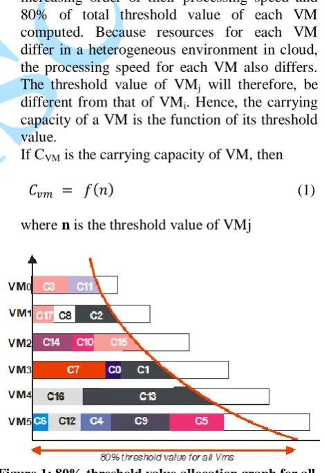
Lower response and turnaround time, higher throughput and efficient VM monitoring capability is the aim of this proposed algorithm. The algorithm is built in a manner that cloudlets allocation to VMs is on the basis of their processing capacities. Eighty per cent of the total threshold value of a virtual machine is considered the best carrying capacity for effective load balancing. In a case where all VMs in the DC have attained 80% of their total threshold value; the remaining 20% of each machine in the DC can then be utilized. This system is built in three phases, (a) VM categorization phase, (b) allocation phase and (c) VM reliability assessment phase. a. VM Categorization Phase:- VMs created and
mapped to physical host(s) in DC are re-arranged by the proposed load balancer in increasing order of their processing speed and 80% of total threshold value of each VM computed. Because resources for each VM differ in a heterogeneous environment in cloud, the processing speed for each VM also differs. The threshold value of VMj will therefore, be
different from that of VMi. Hence, the carrying
capacity of a VM is the function of its threshold value.
If CVM is the carrying capacity of VM, then
(1)
where n is the threshold value of VMj
Figure 1: 80% threshold value allocation graph for all VMs
attained this boundary and there are still cloudlets in the global queue.
b. Allocation Phase:- A VM is considered suitable for cloudlet allocation if it satisfies two conditions. Cloudlet computation time is not more than 80% threshold value of the machine and the VM is lightly loaded. As datacentre controller queries the load balancer for cloudlet allocation, the load balancer measures the length (in million instructions) of the cloudlet and accordingly chooses a VM (termed corresponding VM) following the two conditions mentioned earlier. There are two possible cases with this allocation.
Best case – The best case scenario is when the cloudlet size is less than 80% threshold value and VM is lightly loaded. In this case, the load balancer allocates the cloudlet to the corresponding VM.
Worst case – A case where cloudlet size is greater than 80% threshold value or no lightly loaded VM. In this case, the load balancer allocates the cloudlet to any VM provided the cloudlet size does not exceed total threshold value of the corresponding VM.
c. Reliability Assessment Phase:- Reliability assessment algorithm is added to this proposed system to monitor the efficiency of each VM. Initially, reliability (R) of each VM is set to 0. We have adaptability factor AF, which is the number of allocations per cycle. A cycle is equivalent to 10 different allocations made to each VM. AF is set to 10 at first allocation to a VM and decremented with subsequent allocations. This implies that 10 ≥ AF ≥ 1. How to calculate Reliability Assessment (RA) for each VMj
From the analysis of the proposed system we have that;
(2)
(3) Where is a constant representing additional computation time for processing a cloudlet.
To obtain turnaround time (TAT) for a particular cloudlet, we first calculate from eq(3) and add the value to the total cloudlet burst time. That will give us the expected TAT for processing the cloudlet. Assume a cloudlet with a burst time (BT) of say 9ms is allocated to VMj whose threshold value is 15ms.
From equation (3) we have;
Hence, TAT = cloudlet burst time + = 9ms + 0.75ms = 9.75ms
At the end of execution of that cloudlet, if TAT ≤ 9.75ms, then R = 1, AF will be decremented if another allocation to same VMj is made.
At AF = 0 we compute Reliability Assessment (RA)
(4)
If RA ≥ 80%, then VMj is efficient. More allocations
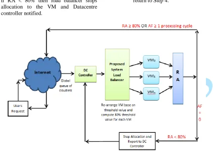
can be made to same VM. AF is initialized back to 10, R is set to 0. If RA < 80%, the load balancer stops allocation to the corresponding VM and notify the datacentre controller. Figure 2 describes the working model of our proposed system.
From Figure 2, all VM from datacentre controller are re-arranged in order of their threshold values. The proposed algorithm maintains an index table with VM id, threshold values, number of cloudlets allocated, reliability (R) and adaptability factor (AF). To measure VM efficiency, reliability assessment module is used. Once the reliability of a machine is less than 80% of its total allocations, the load balancer stops allocating cloudlets to such VM and a notification is sent to the datacentre controller. Steps involved in our proposed system are described below.
Step 1: Re-arrange VMs in increasing order of their threshold value and calculate 80% total threshold value for each VM.
Step 2: Data centre controller received a new request
Step 3: Allocation count set as 0: AF = 10
Step 4: Datacentre controller queries load balancer for allocation of cloudlet
Step 5: Load balancer checks VM whose 80% threshold value is greater than or equal to cloudlet size.
Step 6: Load balancer returns the VM id to datacentre controller
Step 7: Datacentre controller notifies load balancer of new allocation
Step 8: Current active load on that VM is modified in the allocation table
Step 9: Allocation count for that VM is incremented by 1
Step 10: VM completes execution and Datacentre controller notifies load balancer of VM de-allocation
Step 12: Adaptability factor (AF) is decremented by 1 Step 13: Reliability assessment is computed
Step 14: if RA < 80% then load balancer stops allocation to the VM and Datacentre controller notified.
Step 15: Datacentre controller checks if there are waiting cloudlets in the queue. If true, then return to Step 4.
Figure 2: Working model of the proposed system
3.1 Hypothetical illustration of the proposed algorithm
To illustrate the working methodology of our proposed system, we assume a reference stream of five cloudlets with their varying burst time in (million instructions) as shown in Table 2 is used. To make this illustration simple, we also assume a single VM with processing time of 7ms. Two performance parameters are taken into account to compare and analyse the algorithm – Average Waiting Time (AWT) and Average Turnaround Time (ATAT). Result of computation in shown in Table 3.
Table 2: Cloudlets Burst Time
Cloudlets Burst time (ms)
C1 3
C2 6
C3 4
C4 5
C5 2
3.1.1 To calculate AWT and ATAT for RRA, we assume a quantum size of 2ms
C1 C2 C3 C4 C5 C1 C2 C3 C4 C2 C4
0 2 4 6 7 9 10 12 14 16 18 20
WT for C1 = 0 + (9 – 2) = 0 + 7 = 7ms
WT for C2 = 2 + (10 - 4) = 2 + 6 = 8ms
WT for C3 = 4 + (12 – 6) = 4 + 6 = 10ms
WT for C4 = 6 + (14 – 7) + (18 – 16) = 6 + 7 + 2 =
15ms
WT for C5 = 7ms
AWT = (7 + 8 + 10 + 15 + 7) / 5 = 47/5 = 9.4ms
TAT for C1 = 10ms
TAT for C2 = 12ms
TAT for C3 = 14ms
TAT for C4 = 20ms
TAT for C5 = 9ms
ATAT = (10 + 12 + 14 + 20 + 9) / 5 = 65/5 =
13.0ms
3.1.2 To calculate AWT and ATAT for the Proposed System
From analysis of the proposed algorithm, if processing time of VM under consideration is 7ms, then its 80% threshold value will be 5.6ms. Therefore, any cloudlet with burst time greater than 5.6ms will have to wait until cloudlets with smaller burst time are executed. The grant chant below shows the execution pattern for all cloudlets.
C1 C3 C4 C5 C2
WT for C1 = 0ms
WT for C2 = 14ms
WT for C3 = 3ms
WT for C4 = 7ms
WT for C5 = 12ms
AWT = (0 + 14 + 3 + 7 + 12) / 5 = 36/5 = 7.2ms
TAT for C1 = 3ms
TAT for C2 = 20ms
TAT for C3 = 7ms
TAT for C4 = 12ms
TAT for C5 = 14ms
ATAT = (3 + 20 + 7 + 12 + 14) / 5 = 56/5 = 11.2ms
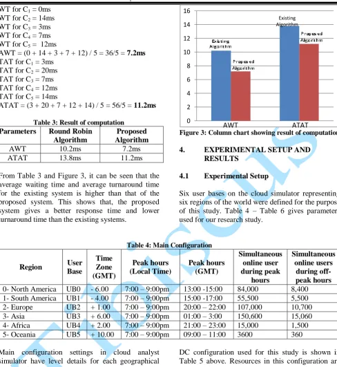
Table 3: Result of computation
Parameters Round Robin
Algorithm
Proposed Algorithm
AWT 10.2ms 7.2ms
ATAT 13.8ms 11.2ms
From Table 3 and Figure 3, it can be seen that the average waiting time and average turnaround time for the existing system is higher than that of the proposed system. This shows that, the proposed system gives a better response time and lower turnaround time than the existing systems.
Figure 3: Column chart showing result of computation
4. EXPERIMENTAL SETUP AND
RESULTS
4.1 Experimental Setup
Six user bases on the cloud simulator representing six regions of the world were defined for the purpose of this study. Table 4 – Table 6 gives parameters used for our research study.
Table 4: Main Configuration
Region User
Base
Time Zone (GMT)
Peak hours (Local Time)
Peak hours (GMT)
Simultaneous online user during peak
hours
Simultaneous online users
during off-peak hours
0- North America UB0 - 6.00 7:00 – 9:00pm 13:00 -15:00 84,000 8,400 1- South America UB1 - 4.00 7:00 – 9:00pm 15:00 -17:00 55,500 5,500 2- Europe UB2 + 1.00 7:00 – 9:00pm 20:00 – 22:00 107,000 10,700 3- Asia UB3 + 6.00 7:00 – 9:00pm 01:00 – 3:00 150,600 15,060 4- Africa UB4 + 2.00 7:00 – 9:00pm 21:00 – 23:00 15,000 1,500 5- Oceania UB5 + 10.00 7:00 – 9:00pm 09:00 – 11:00 3600 360
Main configuration settings in cloud analyst simulator have level details for each geographical region of the world. Table 4 shows these main configurations to be used for this study. The parameters used in this configuration are taken into consideration as a data set from social network site - facebook.
Table 5: Data centre configuration
Parameters Value used
VM image size 10,000
VM memory 512MB
VM bandwidth 1000
DC - Architecture x86
DC - OS Linux
DC - VMM Xen
DC - Number of machine 5
DC configuration used for this study is shown in Table 5 above. Resources in this configuration are DC architecture, operating system of the host machine inside server farm of associated DC. Xen virtual machine monitor is used to monitor virtualization control.
Table 6: Physical hardware details of DC
Parameters Value used
DC - memory per machine 1,024MB
DC - storage per machine 100,000 DC - available bandwidth per machine 10,000 DC - number of processors per machine 3
DC - processor speed 100MIPS
DC - VM policy Time-Shared
DC - User grouping tables in user base 1000 DC - request grouping factor 100 DC - Executable instruction length per request 250 bytes
0 2 4 6 8 10 12 14 16
Proposed Algorithm Existing
Algorithm
AWT
ATAT ATAT
Details of each VM in DC are captured in Table 6. The memory, storage and bandwidth per machine are detailed in this table. For the purpose of simulation, we make some assumptions on the data set.
i. A single time zone has been considered for each user base.
ii. Most people use facebook in the evening after returning from their place of work for at least 2 hours.
iii. 5% of the total registered facebook users of our hypothetical application remain active during peak hours and 10% of the peak hour users remain online in off-peak hours. Table 4 to 6 simply prepare our work for simulation by setting the parameters at infrastructure, platform and user level.
5. RESULT/COMPARISON
Like with most real-world web applications, the two algorithms were run differently on a cloud analyst simulator deployed in a single location, in region (Africa) taking into consideration diverse scenarios. The first scenario assumed a case where cloudlets are deployed on a single datacentre with 20VMs in region 5 (Africa). Other scenarios have same number of VMs each deployed on 2, 3, 4 and 5 datacentres respectively. The physical hardware details of DC still remains as in Table 6 with 1,024MB of memory in each VM running on physical processors capable of speed of 100MIPS.
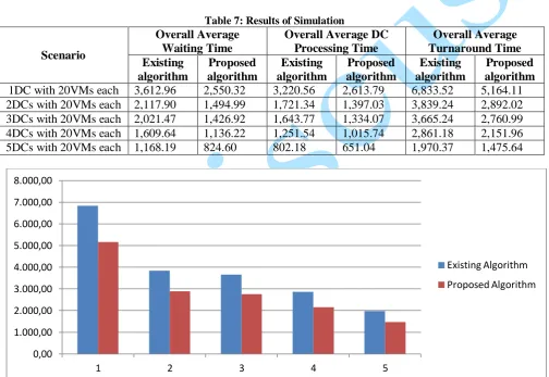
Table 7: Results of Simulation
Scenario
Overall Average Waiting Time
Overall Average DC Processing Time
Overall Average Turnaround Time Existing
algorithm
Proposed algorithm
Existing algorithm
Proposed algorithm
Existing algorithm
Proposed algorithm
1DC with 20VMs each 3,612.96 2,550.32 3,220.56 2,613.79 6,833.52 5,164.11 2DCs with 20VMs each 2,117.90 1,494.99 1,721.34 1,397.03 3,839.24 2,892.02 3DCs with 20VMs each 2,021.47 1,426.92 1,643.77 1,334.07 3,665.24 2,760.99 4DCs with 20VMs each 1,609.64 1,136.22 1,251.54 1,015.74 2,861.18 2,151.96 5DCs with 20VMs each 1,168.19 824.60 802.18 651.04 1,970.37 1,475.64
Figure 4: Column chart showing the overall average turnaround time for both existing and proposed algorithms
As shown in Table 7, simulation results used for comparison are based on the following:
i. Overall Average Waiting Time (time it takes to respond to each task)
ii. Overall Average Datacenter Processing Time (time it takes to complete a task)
iii. Overall Average Turnaround Time (waiting time + processing time)
5.1 Discussion
A careful observation of Table 7 and Figure 4 shows that with a single datacentre, the proposed algorithm shows a very significant difference from the existing algorithm. The results of both algorithms dropped as more datacentres are added to execute cloudlets. Though significant difference still exist between the two algorithms as more datacenters are added, it is possible that with a greater number of datacenters and same number of virtual machines, there may not be major difference between the two algorithms. The 0,00
1.000,00 2.000,00 3.000,00 4.000,00 5.000,00 6.000,00 7.000,00 8.000,00
1 2 3 4 5
Existing Algorithm
proposed VM load balancer however, gives a better result than the existing round robin VM load balancer.
5.2 Conclusion
This research work proposed an enhanced round robin load balancer for cloud infrastructure. The improved model is built with three phases; VM categorization phase for re-arranging VM based on processing speed and 80% threshold value, allocation phase for resource allocation to cloudlets and the reliability assessment phase for efficient VM monitoring. The proposed algorithm shows that 80% of the total threshold value of each VM is considered the best carrying capacity for each VM. A worst case scenario is when all VMs in the DC have attained 80% of their total threshold value; then the algorithm utilizes the remaining 20% of each machine in the DC. A hypothetical illustration and extensive simulation using cloud analyst simulator was carried out and the results shows that the proposed VM load balancer performs better that the existing round robin load balancer. 80% of total threshold value has been proven as a best case scenario for our design if each VM will yield better response time and higher throughput. Results from Table 8 shows that the proposed algorithm yields better response and turnaround time when compared to the existing throttled virtual machine load balancer.
REFERENCES
[AR16] Akbari M., Rashidi H. - A multi-objectives scheduling algorithm based on cuckoo optimization for task allocation problem at compile time in heterogeneous systems. Expert Systems with Applications, Vol. 60, pp. 234– 248, 2016.
[ASS15] Amin Z., Sethi N., Singh H. - Review on fault tolerance techniques in cloud computing. International Journal of Computer Application, Vol. 116, No. 18, pp. 11-16, 2015.
[BRR09] Bhathiya W., Rodrigo N. C., Rajkumar B. - CloudAnalyst: A CloudSim-based Visual Modeller for Analysing Cloud Computing Environments and Applications. Technical Report, CLOUDS-TR-2009-12, Cloud Computing and Distributed Systems Laboratory, The University of Melbourne, Australia, 2009.
[H+17] Hajara I., Absalom E. E., Sahalu B. J., Aderemi O. A. - An improved ant
colony optimization algorithm with fault tolerance for job scheduling in grid computing systems. PLoS ONE,
12(5): e0177567.
https://doi.org/10.1371/journal.pone.01 77567, 2017.
[J+11] Junjie N., Yuanqiang H., Zhongzhi L., Juncheng Z., Depei Q. - Virtual machine mapping policy based on load balancing in private cloud environment, International Conference on Cloud and Service Computing (CSC). pp. 292-295, 2011.
[KAD13] Komal M., Ansuyia M., Deepak D. - Round Robin with Server Affinity: A VM Load Balancing Algorithm for Cloud Based Infrastructure. J Inf Process Syst. Vol. 9, No. 3, pp. 379-392, 2013.
[MM13] Mayanka K., Mishra A. - A comparative study of load balancing algorithms in cloud computing environment. International Journal of Distributed and Cloud Computing. Vol. 1, Issue 2, pp. 1-12, 2013.
[N+12] Nishant K. P., Sharma V., Krishna C., Gupta K. P., Singh N., Nitin, Rastogi R. - Load Balancing of Nodes in Cloud Using Ant Colony Optimization. In Proc. 14th International Conference on Computer Modelling and Simulation (UKSim), IEEE, pp. 3-8, 2012.
[RH15] Rasti-Barzoki M., Hejazi R. S. - Pseudo-polynomial dynamic programming for an integrated due date assignment, resource allocation, production, and distribution scheduling model in supply chain scheduling. Applied Mathematical Modelling, Vol. 39, No. 12, pp. 3280–3289, 2015. [REL09] Rimal B. P., Eunmi C., Lumb I. - A
Taxonomy and Survey of Cloud Computing Systems, Fifth International Joint Conference on Cloud Computing. pp. 44-51, 2009.
[Ver10] Versace M. - NIST defines cloud computing. Retrieved from