Numerical solution of Convection-Diffusion equations with memory
term based on sinc method
Atefeh Fahim
Department of Mathematics, Central Tehran Branch, Islamic Azad University, Tehran, Iran.
E-mail: [email protected]
Mohammad Ali Fariborzi Araghi∗
Department of Mathematics, Central Tehran Branch, Islamic Azad University, Tehran, Iran.
E-mail: [email protected]
Abstract In this essay, we study the numerical solution of Convection-Diffusion equation with a memory term subject to initial boundary value conditions. Finite difference method in combination with product trapezoidal integration rule is used to discretize the equation in time and sinc collocation method is employed in space. The accuracy and error analysis of the method are discussed. Numerical examples and illustrations are presented to prove the validity of the suggested method.
Keywords. Partial integro-differential equation, Sinc collocation method, Finite difference method, Prod-uct trapezoidal integration rule, Convection-diffusion equation.
2010 Mathematics Subject Classification. 65R99, 45A99, 45K05.
1. Introduction
We consider convection-diffusion equation with memory term of the form [10]
ut(x, t) +mux(x, t)−buxx(x, t) =
∫ t
0
k0(t−s)u(x, s)ds+f(x, t),
x∈Ω = [0,1], t∈J = [0, T]. (1.1)
Subjected to initial and boundary conditions,
u(0, t) = u(1, t) = 0, t∈J,
u(x,0) = u0(x), x∈Ω, (1.2)
wherem>0 andb >0 are constants quantity that are denoted the advection(convection) and diffusion processes, respectively. Here ut = ∂u∂t, ux = ∂u∂x, uxx = ∂
2u
∂x2, k0 is
as-sumed to be weakly singular kernel, i.e. satisfiesk0(t) =t−β, 0< β <1 and f is a
given smooth function.
Received: 19 June 2017 ; Accepted: 12 May 2018.
∗Corresponding author.
When the effects of the memory in the system are considered, the model involves the integral or partial differential operator containing the unknown function. Thus, the arising equation appears as partial integro-differential equation (PIDE), consists of partial differentiations and integral terms that is well known as memory term. Model-ing phenomena in viscoelasticity, biological models, chemical kinetics, heat conduction in materials with memory, population dynamics, fluid dynamics and nuclear reactor dynamics, mathematical biology, financial mathematics, compression of visco-elastic media, and other similar areas are all done by partial integro-differential equations. See for example [4,8] and the references cited within.
The convection-diffusion equation is a parabolic partial differential equation, which describes physical phenomena where the energy is transformed inside a physical sys-tem due to two processes, convection and diffusion. This takes place when the integral term in Eq. (1.1) is zero. When, it is necessary analyzed a heat transfer system where high-temperature gas passes through a porous medium placed in a duct, and showed that the porous medium can effectively convert the gas enthalpy into thermal ra-diation, convection-diffusion with memory term of the form Eq. (1.1) is performed [2,15].
Partial integro-differential equations such as Eq. (1.1) are usually difficult to solve analytically. So, it is required to obtain an efficient approximate solution with use of numerical methods. One idea to solve Eq. (1.1) is discretization of the equation in time and spatial directions numerically. Sidiqqi and Arshed [10], used backward Euler method in combination with Euler’s product integration rule in time and cubic B-spline collocation method in space. In Euler’s product integration rule, a weakly singular integral, replaced with a quadrature formula that approximated the integrand by a piecewise constant function agreeing with the integrand at the left endpoint of each subinterval and an error of magnitude isO(∆t) [5].
In this paper, we apply the backward Euler method in time direction and in addi-tion using product trapezoidal integraaddi-tion rule [5], for integral term. Consequently, Eq.(1.1) reduced to a system of ordinary differential equations (ODEs) that is dis-cretized with sinc collocation method. In addition, the accuracy and efficiency of the suggested method will be tested with some examples and illustrations and compared with the method of Sidiqqi and Arshed [10].
The organization of this paper is as follows. Section 2, contains some notations, definitions, assumptions and preliminaries of sinc approximation. The description of the method in order to discrete Convection-Diffusion equation with memory term is devoted in two subsections in section 3. In section 4, the error analysis of the method is described in detail. Finally, in section 5, numerical examples are solved to verify the accuracy and efficiency of the proposed approach.
2. Preliminaries
Sinc method is defined on the real line basically. So, for anyh >0, the translated sinc functions with evenly spaced nodes are given as
S(j, h) (z) = sinc (
z−jh
h
)
, j = 0,±1,±2, . . . , (2.1)
where, the sinc function is defined by
sinc (z) =
{ sin(πz)
πz , z̸= 0,
1, z= 0.
The sinc function for the interpolating pointsxk=khis given by
S(j, h) (kh) =δ(0)jk =
{
1, k=j,
0, k̸=j.
They are based on the infinite stripDd in the complex plane
Dd=
{
w=u+iv:|v|< d≤π
2 }
.
Letf be a function defined on R, andh > 0 is the mesh size, then the Whittaker Cardinal function [11] is defined by the infinite series as follows:
C(f, h, x) =
∞
∑
j=−∞
f(jh)S(j, h)(x). (2.2)
But in practical, in order to coding the finite number of terms are used in the above series such asj=−N, ..., N, where 2N+ 1 is the number of sinc grid points. So, the approximation of Eq. (2.2) is rewritten as
C(f, h, x)≈
N
∑
j=−N
f(jh)S(j, h)(x),
where h suitably selected depending on properties of the function f and a given positive integerN.
To construct an approximation on the interval Γ = (a, b), we consider the conformal map
ϕ(z) = log (
z−a
b−z
)
. (2.3)
The mapϕcarries the eye-shaped region
DE =
{
z=x+ –iy:arg
(
z−a
b−z
)
< d6 π
2,–i
2=−1
}
,
ontoDd such thatϕ(a) =−∞, ϕ(b) =∞, wherea, bare boundary points ofDEwith
a, b∈∂DE. For the sinc method on the interval Γ = (a, b), basis functions are from
the composite translated sinc functions,
Sj(z) =S(j, h)◦(ϕ(z)) = sinc
(
ϕ(z)−jh
h
)
The inverse map ofw=ϕ(z) is
z=ϕ−1(w) =a+be
w
1 +ew .
Letψ denote the inverse map ofϕ, so we define the range ofϕ−1on the real line as
Γ ={ψ(u) =ϕ−1(u)∈DE:−∞< u <∞
}
= (a, b).
Forh >0, let the pointsxk on Γ given by
xk =ψ(kh) =
a+bekh
1 +ekh , k∈Z. (2.4)
Definition 2.1. ([13]) Let Lα(DE) be the set of all analytic functions f, for which
there exists a constant,C, such that
|f(z)| ≤C |ρ(z)|
α
(1 +|ρ(z)|)2α, z∈DE, 0< α≤1, (2.5)
whereρ(z) =eϕ(z).
Definition 2.2. ([11]) LetB(DE) is the class of functions f which are analytic in
DE such that
∫
ψ(u+∑)
|f(z)| |dz| →0, as u→ ±∞,
where∑={–iη:|η|< d6π2,–i2=−1}and satisfy
ℵ(f)≡ ∫
∂DE
|f(z)| |dz|<∞,
where∂DE represents the boundary of DE.
Theorem 2.3. ([13]) Let F ∈ Lα(DE), let N be a positive integer, and let h be
selected by the formula
h= √c
N,
withc a positive constant. Then there exist positive constants C andκ, independent ofN, such that
sup
z∈Γ
F(z)−
N
∑
k=−N
F(zk)S(k, h)◦ϕ(z)
6Ce−κ
√ N.
The sinc collocation method requires that the derivatives of composite sinc function be evaluated at the nodes. So, we need to recall the following lemma.
Lemma 2.4. ([6], p. 106) Letϕbe the conformal one-to-one mapping of the simply connected domainDE ontoDd , given by (2.3). Then
δjk(0)= [S(j, h)◦ϕ(x)]|x=x
k=
{1, j=k,
δjk(1)=h d
dϕ[S(j, h)◦ϕ(x)]|x=xk=
0, j=k,
(−1)k−j
k−j , j̸=k,
(2.7)
δjk(2)=h2 d
2
dϕ2[S(j, h)◦ϕ(x)]|x=xk =
−π2
3 , j=k,
−2(−1)k−j
(k−j)2 , j̸=k.
(2.8)
In Eqs. (2.6)-(2.8),his step size andxk is sinc grid given by (2.4).
3. Description of the method
In this section, a description of the spatial-temporal discretization about this type of equations is provided in detail.
3.1. Discretization in time: The backward Euler method is applied for time-derivatives in Eq. (1.1). Lettn=n∆twith ∆t= KT, K∈Nbeing the time step andun =u(x, tn)
andfn=f(x, tn) forn= 0,1, ..., M,16M 6K. By replacingt=tn+1 into the left
hand side of Eq. (1.1) for the first term we get
ut(x, tn+1)≈
un+1(x)−un(x)
∆t , 0< x <1, n>0, (3.1)
and the integral term of (1.1) can be approximated by the product trapezoidal inte-gration rule [5] as follows:
∫ tn+1
0
(tn+1−s)− β
u(x, s)ds=
n
∑
l=0
∫ tl+1
tl
(tn+1−s)− β
u(x, s)ds
≈ n
∑
l=0
∫ tl+1
tl
(tn+1−s)− β
{
tl+1−s
∆t u
l(x) +s−tl
∆t u
l+1(x)
}
ds
= 1 ∆t
n
∑
l=0
(
λn,lul(x) +ηn,lul+1(x)
)
, (3.2)
where,
λn,l =
∫ tl+1
tl
(tn+1−s)−β(tl+1−s)ds,
ηn,l =
∫ tl+1
tl
(tn+1−s)− β
Substituting Eqs. (3.1) and Eq. (3.2) into Eq. (1.1), we can get the temporal semi-discrete form of Eq. (1.1), as follows:
(1−ηn,n)un+1(x) + ∆t
(
mun+1
x (x)−bun+1xx (x)
)
=un(x) + ∆tfn+1(x) +
n
∑
l=0
ρn,lul(x),0< x <1, n>0, (3.4)
un+1(0) = 0, un+1(1) = 0, (3.5)
where,
ρn,0 = λn,0,
ρn,l = λn,l+ηn,l−1, l= 1,2, . . . , n, (3.6)
and with additional initial condition
u0(x) =u0(x).
As a consequence, a linear ordinary differential equation is obtained in the form of (3.4) with boundary conditions (3.5) in each time level. Now, we can use the sinc collocation method to estimate the solution of this linear boundary value problem.
3.2. Discretization in space: We discretize the spatial direction by the described sinc collocation method. Assume that the approximate solution of (3.4) defined by
unm(x) =
N
∑
j=−N
cnjS(j, h)◦ϕ(x), m= 2N+ 1, (3.7)
and
ϕ(x) = log( x 1−x),
and the unknown coefficientcn
j in Eq. (3.7) are determined by sinc collocation method.
The collocation points are as
xi=
eih
1 +eih, i=−N, ..., N, h=
c
√
N, (3.8)
so,
d
dxu
n
m(x) = N
∑
j=−N
cnj
d
dx[S(j, h)◦ϕ(x)]
=
N
∑
j=−N
cnj
[
ϕ′(x)Sj(1)(x) ]
, (3.9)
and,
d2
dx2u
n
m(x) = N
∑
j=−N
cnj d
2
dx2[S(j, h)◦ϕ(x)]
=
N
∑
j=−N
cnj
[
ϕ′′(x)Sj(1)(x) + (ϕ′(x))2Sj(2)(x) ]
where,
Sj(l)(x) = d
l
dϕl[S(j, h)◦ϕ(x)], l= 1,2,
thus, by applying notations in Lemma (2.4),
d
dxu
n m(xi) =
N
∑
j=−N
cnj
[
ϕ′(xi)
δ(1)ji h
]
, (3.11)
and,
d2
dx2u
n m(xi) =
N
∑
j=−N
cnj
[
ϕ′′(xi)
δji(1)
h + (ϕ
′(x i)) 2δ (2) ji h2 ] . (3.12)
Substituting (3.7), (3.11) and (3.12) into (3.4) we obtain,
(1−ηn,n) N
∑
j=−N
cn+1j δji(0)+m∆t
N
∑
j=−N
cn+1j
[
ϕ′(xi)
δji(1) h
]
−b∆t
N
∑
j=−N
cn+1j
[
ϕ′′(xi)
δ(1)ji
h + (ϕ
′(x i)) 2δ (2) ji h2 ]
=cni + ∆tfin+1+
n
∑
l=0 N
∑
j=−N
ρn,lcljδ (0)
ji , (3.13)
with additional initial condition,
c0i =u0(xi), i=−N, . . . , N. (3.14)
We note thatδ(0)ji =δij(0), δji(1) =−δij(1) andδji(2) =δ(2)ij . We denote I(r)= [δ(r) ij ], r =
0,1,2 whereI(0) is identity matrix andI(1),I(2) are symmetric and skew-symmetric
Toplitz matrix of order 2N + 1 respectively. We define the (2N + 1)×(2N + 1) diagonal matrix as follows:
D(g(x))ij=
{
g(xi), i=j,
0, i̸=j. (3.15)
By multiplying both sides of (3.13) in (ϕ′(x1
i))2 we conclude
(1−ηn,n)
( 1
(ϕ′(xi)) 2
)
cn+1i −m∆t
N
∑
j=−N
[( 1
ϕ′(xi)
)δ(1) ij
h
]
cn+1j
−b∆t
N
∑
j=−N
[(
−ϕ′′(xi)
(ϕ′(xi)) 2
)
δij(1)
h +
δij(2)
h2
]
cn+1j
= (
1
(ϕ′(xi)) 2
)
cni + ∆t
( 1
(ϕ′(xi)) 2
)
fin+1+
n ∑ l=0 ρn,l ( 1
(ϕ′(xi)) 2
)
Therefore, the system (3.16) can be denoted by the following matrix form:
P Cn+1=Q, (3.17)
where,
P = (1−ηn,n)D ((
1
ϕ′ )2)
I(0)−∆t (
m hD
(
1
ϕ′ )
+b
hD ((
1
ϕ′ )′)
I(1)+ b
h2I (2)
) ,
Q=D
(( 1
ϕ′
)2)(
Cn+ ∆tFn+1)+
n
∑
l=0
ρn,lD
(( 1
ϕ′
)2)
Cl, (3.18)
and,
Cn+1 = (cn+1−N, cn+1−N+1, . . . , cn+1N )t,
Fn+1 = (f−n+1N , f−n+1N+1, . . . , fNn+1)t, (3.19)
with additional initial condition,
C0= (u0(x−N), u0(x−N+1), . . . , u0(xN))
t
. (3.20)
For eachn, system (3.17) is a linear system of equations which consists of 2N+ 1 equations and 2N + 1 unknowns. The coefficients cn
j, in the approximate solution
(3.7), can be determined by solving (3.17).
4. Error Analysis
When we apply backward Euler method in Eq. (1.1), ut and integral term are
approximated as follow:
ut(x, tn+1)≈
un+1(x)−un(x)
∆t +O(∆t), (4.1)
and, ∫ tn+1
0
(tn+1−s)− β
u(x, s)ds≈ 1
∆t
n
∑
l=0
(
λn,lul+ηn,lul+1
)
+O(∆t2−β), (4.2)
the order of product trapezoidal integration rule isO(∆t2−β) that is proved by Dixon in [1].
Lemma 4.1. [3] The following estimates hold
u(x, t)≈u(xi, t) +C1e−κ
√ N,
ux(x, t)≈ux(xi, t) +C2e−κ
√ N,
uxx(x, t)≈uxx(xi, t) +C3e−κ
√ N,
whereκ >0,−N 6i6N,C1,C2, andC3 are constants independent ofN.
Theorem 4.2. By using the finite difference method and product integration rule in combination with sinccollocation method the truncation error of the proposed ap-proach isO((∆t) +e−κ√N).
Proof. Replacing Eqs. (4.1) and (4.2) into Eq. (1.1) and discretization in time, we obtain,
ut(x, tn+1) +O(∆t)−
∫ tn+1
0
(tn+1−s)−βu(x, s)ds+O
(
∆t2−β)=χ(x, tn+1), (4.3)
where,
χ(x, t) =f(x, t)−mux(x, t) +buxx(x, t). (4.4)
From lemma 4.1 and discretization in spatial direction,
χ(xi, tn+1) =f(xi, tn+1)−m
(
ux(xi, tn+1) +c1e−κ √
N)
+b (
uxx(xi, tn+1) +c2e−κ √
N) ,(4.5)
if we suppose that the truncation error estimated as
T E(x, t) =ut−
∫ t
0
(t−s)−βu(x, s)ds−χ(x, t),
then,
T E(xi, tn+1) =O(∆t) +O
(
∆t2−β)+ (mc1−bc2)e−κ √
N,
Algorithm 1
1: InputT, K, M, N, u0(x), f(x, t), uex(x, t),
2: Setxi:=
eih
1 +eih, i=−N, ..., N, zk:=kp, k= 0, . . . , N,
3: Settj :=j∆t, j= 0,1, ..., M,
4: Computeuex(xi, tj), uex(zk, tj),
5: Computeuapp(xi, tj), as follows:
6: Setuapp(xi, t0) :=c0i, i=−N, ..., N, based on Eq. (3.20)
forj= 0 :M−1 do fori=−N :N do
uapp(xi, tj+1) :=cj+1i ,by applying Eqs. (3.17) and (3.18)
end do end do
7: Setuapp(zk, tM) :=
∑N j=−Nc
M
j S(j, h)◦ϕ(zk),by applying (3.7)
8: error1(i) :=|uex(xi, tM)−uapp(xi, tM)|, i=−N, ..., N,
error2(k) :=|uex(zk, tM)−uapp(zk, tM)|, k= 0, ..., N,
error3 := 2N1+1(∑Ni=−N|uapp(xi, tM)−uex(xi, tM)|2)
1 2,
error4 := N1+1(∑Nk=0|uapp(zk, tM)−uex(zk, tM)|2)
1 2,
9: Print∥EM∥∞:=max(error1(i)), i=−N, ..., N,
Print∥eM∥∞:=max(error2(k)), k= 0, ..., N,
Print∥EM∥2:=error3,
Print∥eM∥2:=error4.
5. Numerical Results
In this section, the numerical experiments of the proposed approach are pro-vided. In all examples, we set parameters c = √πd/α, d = π2 and α = 1 and denote computed solution and exact solution by uapp and uex, respectively. Let
tn = n∆t, n = 0,1, . . . , M, which M denotes the last time tM and ∆t is the small
time step. The maximum error norm and Euclidian error norm in pointszk=kp, k=
0,1, ..., N, p= N1 between the computed and exact solutions are given as∥eM∥∞and
∥eM∥2, respectively. Also, the maximum error norm and Euclidian error norm in
pointsxi = e
ih
1+eih, i=−N, ..., N, h=
c √
N are given as∥EM∥∞ and ∥EM∥2,
respec-tively as follows:
∥eM∥∞ = M ax
k |uapp(zk, tM)−uex(zk, tM)|, k= 0, . . . , N,
∥EM∥∞ = M ax
i |uapp(xi, tM)−uex(xi, tM)|, i=−N, . . . , N,
∥eM∥2 =
1
N+ 1(
N
∑
k=0
|uapp(zk, tM)−uex(zk, tM)|2)
1 2,
∥EM∥2 =
1 2N+ 1(
N
∑
i=−N
|uapp(xi, tM)−uex(xi, tM)|2)
Table 1. Results of example 1.
∆t= 10−3 ∆t= 10−4 ∆t= 10−5
∥.∥ M proposed approach proposed approach method in [10] proposed approach method in [10] ∥eM∥∞ 10 1.9089E−04 1.5230E−05 2.6417E−05 8.8082E−07 6.7929E−06
50 1.2601E−03 4.2241E−05 3.9890E−05 1.0096E−05 2.0040E−05
100 2.6432E−03 9.0542E−05 4.4030E−05 1.5412E−05 2.6950E−05
500 1.3863E−02 4.8595E−04 5.3632E−05 2.5124E−05 4.0214E−05
∥eM∥2 10 1.8904E−05 7.6715E−07 5.6276E−07 3.1893E−08 1.3756E−07
50 1.2422E−04 4.3127E−06 1.0863E−06 3.1303E−07 4.1125E−07
100 2.6009E−04 9.1029E−06 1.3976E−06 5.3657E−07 5.8715E−07
500 1.3611E−03 4.8350E−05 2.8654E−06 1.8721E−06 1.2581E−06
In order to implement the proposed approach, algorithm 1 is given.
The linear algebraic system in step 6 of algorithm 1 is solved directly by using “linsolve” command from “LinearAlgebra” package in Matlab R2014a software and all the calculations were supported by intel CORE Dual-Core at 2.20 GHz CPU with 4 GB RAM.
Example 1. Consider Eq. (1.1), whenm = 0.05, b = 0.4, β = 12, u0(x) = sin(πx)
and
f(x, t) =
(
2 (1 +t) +bπ2(1 +t)2−2√t (
1 +4 3t+
8 15t
2
))
sin (πx) +mπ(1 +t)2cos (πx).
The analytic solution is given byu(x, t) = (1+t)2sin(πx) [10]. In Table1, maximum and Euclidian error norms of the presented approach with regarding N = 25 are compared with cubic B-spline collocation method in [10] when N = 50, for T = 1 and ∆t = 10−3, ∆t = 10−4 and ∆t = 10−5 in the different time levels tM. This
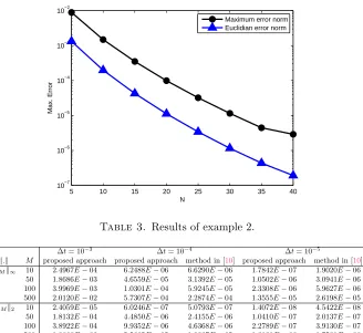
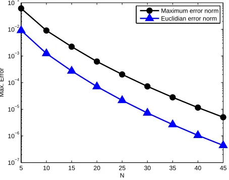
table shows that, the presented approach is in good agreement with the method in [10]. In Table 2, we set ∆t = 10−5 for different values ofN. Results of this table
demonstrate the exponential convergence rate of the proposed approach by increasing values ofN. Furthermore, in this table condition number with use of Euclidian norm and CPU time based on second are reported. Convergence curves of Table 2 are plotted in Figure 1. Based on the idea mentioned in [9], Figure 2 reports that the sinc collocation method achieves an approximation convergence rate because the|c100
j |
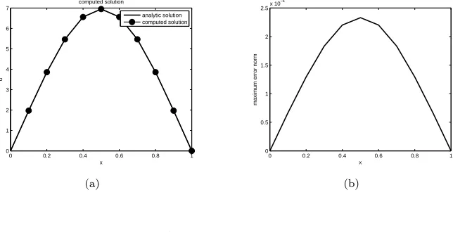
falls off when|j|tends toN and also, shows that ifN is increased, the approximate solution converges to the analytic solution. In addition, the analytic and computed solutions in the different values of x is ploted in Figure 3 (a), and the maximum error norm in the sinc collocation points is ploted in Figure 3 (b) for N = 35 and ∆t= 10−5.
Example 2. Consider Eq. (1.1), when m = 0.005, b = 0.5, β = 1
3, u0(x) =
1−cos (2πx) + 2π2x(1−x) and
f(x, t) =(1−cos (2πx) + 2π2x(1−x)) (2 (t+ 1)−(t+ 1) 2
t1−β
1−β +
2 (t+ 1)t2−β
2−β − t3−β
3−β )
+(2 (m+ 2b)π2−4mπ2x+ 2mπsin (2πx)−4bπ2cos (2πx))(t+ 1)2.
The exact solution is given by [10]
Table 2. Results of example 1 att= 0.001.
∆t= 10−5, M= 100
N ∥EM∥∞ ∥EM∥2 Cond(P) CP U time(s)
5 8.8737×10⁻³ 1.3276×10⁻³ 1.04×10³ 0.093
10 1.4835×10⁻³ 1.9793×10⁻⁴ 6.26×10³ 0.099
15 3.5188×10⁻⁴ 4.2850×10⁻⁵ 1.49×10⁴ 0.104
20 9.9114×10⁻⁵ 1.1222×10⁻⁵ 2.49×10⁴ 17.280
25 3.2173×10⁻⁵ 3.4096×10⁻⁶ 3.50×10⁴ 20.363
30 1.1519×10⁻⁵ 1.1572×10⁻⁶ 4.48×10⁴ 20.912
35 4.4614×10⁻⁶ 4.3661×10⁻⁷ 5.41×10⁴ 34.437
40 2.9079×10⁻⁶ 1.9241×10⁻⁷ 6.28×10⁴ 38.519
Figure 1. Convergence curve for example 1 att= 0.001.
5 10 15 20 25 30 35 40
10−7 10−6 10−5 10−4 10−3 10−2
N
Max. Error
Maximum error norm Euclidian error norm
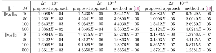
Table 3. Results of example 2.
∆t= 10−3 ∆t= 10−4 ∆t= 10−5
∥.∥ M proposed approach proposed approach method in [10] proposed approach method in [10] ∥eM∥∞ 10 2.4967E−04 6.2488E−06 6.6290E−06 1.7842E−07 1.9020E−06
50 1.8686E−03 4.6559E−05 3.1392E−05 1.0502E−06 3.0941E−06
100 3.9969E−03 1.0301E−04 5.9245E−05 2.3308E−06 5.9627E−06
500 2.0120E−02 5.7307E−04 2.2874E−04 1.3555E−05 2.6198E−05
∥eM∥2 10 2.4059E−05 6.0246E−07 5.0793E−07 1.4072E−08 4.5422E−08
50 1.8132E−04 4.4850E−06 2.4155E−06 1.0410E−07 2.0137E−07
100 3.8922E−04 9.9352E−06 4.6368E−06 2.2789E−07 3.9130E−07
500 1.9666E−03 5.5665E−05 1.9337E−05 1.3121E−06 1.7531E−06
The numerical solutions for N = 50 , T = 1 with ∆t = 10−3, ∆t = 10−4 and
∆t= 10−5 at different time levels t
M of the proposed approach are listed and
Figure 2. Plot of |c100
j | coefficients for example 1 defined by Eq.
(3.7) forN = 5,10,20 and ∆t= 10−5.
−200 −15 −10 −5 0 5 10 15 20
0.2 0.4 0.6 0.8 1 1.2 1.4
N
|cj
100
|
N=5 N=10 N=20
Figure 3. (a) The analytic and computed solutions and (b) the maximum error norm att= 0.001 for example 1.
0 0.2 0.4 0.6 0.8 1 0
0.2 0.4 0.6 0.8 1 1.2 1.4
x
u
analytic solution computed solution
(a)
0 0.2 0.4 0.6 0.8 1 0
0.5 1 1.5 2 2.5
3x 10 −6
x
maximum error norm
(b)
Table 4. Results of example 2 att= 0.001.
∆t= 10−5, M= 100
N ∥EM∥∞ ∥EM∥2 Cond(P) CP U time(s)
5 6.1135×10⁻² 9.1320×10⁻³ 9.90×10² 0.093
10 9.0552×10⁻³ 1.2442×10⁻³ 5.43×10³ 0.101
15 2.2376×10⁻³ 2.7474×10⁻⁴ 1.26×10⁴ 0.110
20 6.1945×10⁻⁴ 7.0968×10⁻⁵ 2.07×10⁴ 0.122
25 2.0268×10⁻⁴ 2.1606×10⁻⁵ 2.89×10⁴ 0.126
30 7.2279×10⁻⁵ 7.2665×10⁻⁶ 3.67×10⁴ 0.127
35 2.8052×10⁻⁵ 2.6709×10⁻⁶ 4.42×10⁴ 0.157
40 1.1546×10⁻⁵ 1.0505×10⁻⁶ 5.12×10⁴ 0.162
45 5.0140×10⁻⁶ 4.4109×10⁻⁷ 5.78×10⁴ 0.210
Figure 4. Convergence curve for example 2 att= 0.001.
5 10 15 20 25 30 35 40 45
10−7 10−6 10−5 10−4 10−3 10−2 10−1
N
Max. Error
Maximum error norm Euclidian error norm
6 (b) the maximum error norm in sinc collocation points is ploted for ∆t = 10−5,
N= 50.
6. Conclusions
In this paper, finite difference method in combination with product trapezoidal integration rule was used to discretize the Convection-Diffusion equation in time. Then, the sinc collocation method was applied to solve outcoming equation in spa-tial direction. To illustrate effectiveness of the given approach, some examples were solved based on the proposed algorithm. Also, the error of the scheme was given. The results show that the proposed approach and the cubic B-spline collocation method for Convection-Diffusion equation are the efficient methods and have a same rather numerical results. Furthermore, the proposed approach is efficient for different values
Figure 5. Plot of |c100
j | coefficients for example 2 defined by Eq.
(3.7) forN = 5,10,20,30 and ∆t= 10−5.
−300 −20 −10 0 10 20 30
1 2 3 4 5 6 7
N |cj
100
|
N=5 N=10 N=20 N=30
Figure 6. (a) The analytic and computed solutions and (b) the maximum error norm for example 2 att= 0.001.
0 0.2 0.4 0.6 0.8 1 0
1 2 3 4 5 6 7
x
u
computed solution
analytic solution computed solution
(a)
0 0.2 0.4 0.6 0.8 1 0
0.5 1 1.5 2 2.5x 10
−6
x
maximum error norm
(b)
Acknowledgment
The authors would like to thank the anonymous reviewers for their constructive comments to improve the quality of this work.
References
[1] J. Dixon,On the order of the error in discretization methods for weakly singular second kind
[2] R. Echigo,Effective energy conversion method between gas enthalpy and thermal radiation and
application to industrial furnaces, Proc. 7th Int. Heat Tratqfer Cont., Miinchen,6(1982), 361–
366.
[3] M. El-Gamel,Error analysis of sinc-Galerkin method for time-dependent partial differential
equations, Numerical Algorithms,77(2) (2018), 517-533.
[4] A. Fasano, A. Mancini, and M. Primicerio, Tumours with cancer stem cells: A PDE model, Mathematical biosciences,272(2016), 76–80.
[5] P. Linz, Analytical and numerical methods for Volterra equations, SIAM Studies in Applied Mathematics, Philadelphia, 1985.
[6] J. Lund and K. L. Bowers,Sinc Methods for Quadrature and Differential Equations, SIAM, Philadelphia, 1992.
[7] J. Ma,Blow-up solutions of nonlinear Volterra integro-differential equations, Mathematical and Computer Modelling,54(11) (2011), 2551–2559.
[8] M. Renardy, W. J. Hrusa, and J. A. Nohel,Mathematical problems in viscoelasticity, Longman Science and Technology, New York, 1987.
[9] A. Saadatmandi, A. Asadi, and A. Eftekhari,Collocation method using quintic B-spline and
sinc functions for solving a model of squeezing flow between two infinite plates, Int. J. Comput.
Math.,93(11) (2016), 1921–1936.
[10] S. Siddiqi and S. Arshad,Numerical solution of convection-diffusion integro-differential
equa-tions with a weakly singular kernel, J. Basic Appl. Sci. Res, 3 (2013), 106–120.
[11] F. Stenger,A sinc-Galerkin method of solution of boundary value problems, Math. Comput.,
33(1979), 85–109.
[12] F. Stenger,Handbook of Sinc Numerical methods, CRC Press, London, 2011.
[13] F. Stenger, Numerical methods based on sinc and analytic functions, Springer Science and Business Media, New York, 1993.
[14] M. Sugihara, Near optimality of the sinc approximation, Mathematics of Computation, 72
(2003), 767–786.
[15] H. Yoshida, J. H. Yun, R. Echigo, and T. Tomimura, Transient characteristics of combined
conduction, convection and radiation heat transfer in porous media, International journal of