in the population sciences published by the Max Planck Institute for Demographic Research Konrad-Zuse Str. 1, D-18057 Rostock · GERMANY www.demographic-research.org
DEMOGRAPHIC RESEARCH
VOLUME 8, ARTICLE 6, PAGES 151-214
PUBLISHED 4 April 2003
www.demographic-research.org/Volumes/Vol8/6/
DOI: 10.4054/DemRes.2003.8.6
Research Article
Tempo-Quantum and Period-Cohort
Interplay in Fertility Changes in Europe.
Evidence from the Czech Republic, Italy,
the Netherlands and Sweden
Tomáš Sobotka
© 2003 Max-Planck-Gesellschaft.
1 Introduction 152 2 Period fertility indicators: Theoretical
considerations
153 2.1 Indicators of period fertility 153 2.2 Attempts to adjust period fertility for tempo
distortions
155 2.3 The meaning of adjusted fertility indicators 157 2.4 Focus of the paper: The proximity of period and
cohort fertility
158 2.5 Timing effects in period fertility: An illustration 159
3 Methods 161
3.1 Linking period and cohort fertility 161 3.2 Indicators of period fertility used in the analysis 162
4 Data 165
5 Four countries, four fertility histories 166 6 Comparison of period and cohort fertility by birth
order
170 6.1 Fertility of birth order 1 170 6.2 Fertility of birth order 2 174 6.3 Fertility of birth order 3 and higher 176 6.4 All births combined: Period indicators of total
fertility
178 7 Additional criteria to analyse the performance of
the period fertility indicators
181 7.1 Approximation of cohort fertility in periods of
intensive postponement
181 7.2 Fluctuations in fertility indicators 183
7.3 ‘Impossible’ cases 184
7.4 Performance in ‘extreme’ situations 184 7.5 Calculating period fertility indicators 185 8 Discussion on the tempo-quantum and
period-cohort interaction
186 9 The use of the alternative period fertility indicators:
Two examples
188 9.1 Estimating tempo and quantum components in
period fertility change
188 9.2 Implications of period fertility trends for cohort
fertility
189
References 199
Appendix 1 204
Appendix 2 207
Appendix 3 211
Research Article
Tempo-Quantum and Period-Cohort Interplay in Fertility Changes
in Europe.
Evidence from the Czech Republic, Italy, the Netherlands and
Sweden
Tomáš Sobotka1
Abstract
Using detailed data on period and cohort fertility in four European countries, this paper discusses various indicators of period fertility, including indicators adjusted for changes in fertility timing. Empirical analysis focuses on the comparison of cohort fertility and corresponding indicators of period fertility; particular attention is paid to the periods of intensive postponement of childbearing. Some period indicators come consistently closer to the completed cohort fertility than the total fertility rates. This pattern of differential period-cohort approximation widely varies by birth order. Quite a high level of approximation is provided by the tempo-adjusted birth probabilities of parity 1 and a combined indicator of total fertility. Two examples illustrate the use of indicators discussed in the paper: the first provides an estimation of the tempo (timing) and quantum (level) components in fertility change in the Czech Republic and the second presents projections of cohort fertility in the Czech Republic and Italy.
1
1. Introduction
Commonly used indicators of period fertility, such as the total fertility rate and age-specific fertility rates, are sensitive to changes in the timing of childbearing among women. During the phases of the timing shifts in fertility schedule – be it either postponement or advancement of births – period fertility measures reflect an interplay of both quantum (level) and tempo (timing) components. Postponement of childbearing has become one of the most characteristic features of fertility trends in Europe at the end of the 20th century. As a result, it has ‘deflated’ the most usual indicator of period fertility, the total fertility rate (TFR), which declined in many countries to extremely low levels. For instance the TFR for birth order 1 has declined below the level of 0.6 in Spain (1995-98), the Czech Republic (1995-2000), Hungary (1997-2000) and Latvia (1997-99). These values do not indicate an unprecedented increase in childlessness, but rather a distinct deferment of births, which has been most intensive in these countries. They also illustrate that due to the postponement of births the TFR has lost its descriptive power as an indicator of period fertility quantum.
Widespread use of the total fertility rates often leads to the misinterpretation of fertility trends, resulting in catastrophic assessments concerning the current level of period fertility as well as the future cohort fertility and their implications for population structure1. What are possible solutions to this problem? A radical solution would be to abandon the use of indicators based on the synthetic cohort2 concept. A less radical solution implies a construction of indicators that provide an adjustment for the distortions present in commonly used fertility measures. In spite of occasional attempts to use alternative indicators, extensive discussion did not start until 1998, when Bongaarts and Feeney proposed a simple adjustment of the total fertility rate, which removes the tempo changes.
This paper investigates whether the use of alternative indicators of period fertility can improve our interpretation of period fertility trends and the projections of future period and cohort fertility. The main question of the paper may be formulated in the following way: Do more elaborate measures of period fertility, by removing some distortions present in the TFR, provide a better approximation of the completed cohort fertility of women who are currently in their childbearing age? This investigation is directly related to the ambiguous questions about the meaning of the period fertility indicators: Do they adequately represent the period trends? Is it possible to make some inferences or projections of the future cohort fertility based on current period fertility measures? Does the use of adjusted fertility indicators improve our understanding of fertility change?
1. To discuss specific issues connected with the use of the synthetic cohort fertility indicators.
2. To analyse trends in period fertility with the use of indicators that are free of some distortions present in the TFR. This analysis is focused primarily on the influences of the tempo effects, in particular the postponement of childbearing.
3. To compare period fertility indicators with the data on completed cohort
fertility and discuss specific advantages and disadvantages of this approach.
4. To illustrate potential benefits of the use of adjusted period fertility
measures.
The analysis is based on period and cohort fertility data for four European countries with different fertility developments: the Czech Republic, Italy, the Netherlands and Sweden. The comparison of period and cohort fertility indicators is performed separately for birth orders 1, 2, and 3+ and for the total fertility.
The paper is divided into ten sections. The Introduction is followed by a theoretical discussion on the period fertility indicators (Section 2). Section 3 provides a description of methods and indicators used, while Section 4 gives an overview of the data. A brief account of recent trends in period and cohort fertility in the four analysed countries is presented in Section 5. Section 6 is focused on the comparison of period and cohort fertility indicators, and further criteria on the use of various period indicators are proposed in Section 7. Section 8 discusses the tempo-quantum and period-cohort interaction, focusing on birth probabilities. Section 9 illustrates some new insights obtained from the use of the adjusted period fertility indicators. The section which follows concludes the paper.
2. Period fertility indicators: Theoretical considerations
2.1. Indicators of period fertility
birth or since marriage). All these indicators may be, with varying degrees of accuracy, derived both from the vital statistics and surveys (for analysis of survey data see Wunsch, 1999). However, national statistical offices usually do not collect data needed for the construction of the more complex fertility measures.
(1) The first and the simplest indicator, the crude birth rate, relates the total number of births in a given year to the total population size. Alternatively, the total number of births may be related only to the number of women of reproductive age (usually given as age 15 to 49). This indicator is called the general fertility rate.
(2) The second approach is based on the age-specific fertility rates (reduced rates, also called frequencies, incidence rates, and rates of the second kind3), which relate number of births women have in a given age group to all women in that age group. The sum of the age-specific fertility rates (ASFR) in a particular year is the total fertility rate. This is a hypothetical indicator, usually interpreted as the average number of children a woman would have if the age-specific fertility rates of a given year remained constant over her reproductive life. The corresponding cohort fertility indicator, summarising the fertility of a cohort born in the same year, is the completed (cohort) fertility rate (CFR). The TFR has several advantages, which account for the widespread use of this indicator. Unlike the crude birth rate, the TFR is not affected by changes in the composition of the female population by age. It can be easily calculated from the data commonly available in all developed countries and as an indicator of the ‘number of children per one woman’ it is intuitively understandable. However, the ASFR are subjected to distortions in fertility timing – postponement or advancement of births and changes in the shape of fertility schedule. When the data on births by birth order are available, the ASFR and the TFR are often computed for each birth order separately. The denominator for the computation of the age and order-specific reduced rates is the population of all women in a given age group. This means that order-specific TFRi are
additive indicators; the sum of the TFRi for different birth orders i gives the TFR.
However, this also implies that the order-specific ASFRi does not discriminate between
women who were exposed to bearing a child of order i (that is, generally, women with i-1 children) and other women. Thus, the order-specific TFRi is frequently distorted by
the parity4 composition of population and its changes over time (Kohler, Billari and
Ortega, 2002: 644-645).
“index controlling for parity and age” (PATFR; Rallu and Toulemon, 1994: 65-67). Childbearing probabilities by parity may be used for a construction of multistate fertility tables, depicting fertility history of the synthetic cohort over its life course (e.g. tables constructed by Bolesławski (1993) for Poland and tables and indicators for Italy (Giorgi, 1993; De Simoni, 1995)). Various indicators of fertility tables were discussed by Park (1976), Willekens (1991) and Ortega and Kohler (2002); the construction of general increment-decrement life tables is described in Schoen (1975). The use of the PATFR concept is limited by the inadequate availability of data on the distribution of women by parity and age. Although the PATFR eliminates the bias of relating births specified by birth order to all women of a given age, which is present in the order-specific TFR and ASFR, it is still subjected to distortions caused by changes in the timing of childbearing among women.
(4) Apart from age and parity, time elapsed since the previous birth or since marriage (duration) is another important variable influencing number of births of a particular birth order. Several researchers (e.g. Ní Bhrolcháin, 1992: 614; Hobcraft, 1993: 450) have suggested that duration since the previous birth should also be included in period fertility indicators. Feeney (1983: 76) has proposed that the “parity progression schedules which incorporate parity progression rates and birth-interval distributions are arguably the most natural approach to the measurement of fertility”. There are examples of complex period fertility indicators using information on age, parity and time since the preceding birth (e.g. Rallu and Toulemon, 1994; Barkalov and Dorbritz, 1996). These data are available only for a few countries and short time periods. Less complex indicators are based only on parity and time since the preceding birth, with the exposure to the first birth analysed since the time of marriage (e.g. Feeney and Yu, 1987; Ní Bhrolcháin, 1987; Brass, 1991).
More detailed overview of various fertility indicators is provided in Rallu and Toulemon (1994), and Ortega and Kohler (2002). The discussion and analysis in this paper focuses on fertility indicators based on reduced rates and birth probabilities. Owing to a lack of data, the indicators based on duration were not included in the analysis5.
2.2. Attempts to adjust period fertility for tempo distortions
and Wales using data on marital fertility by parity and interval since previous birth. Murphy (1994: 53-54) proposed adjustment of the TFR based on changes in the mean age of childbearing (more accurately called the mean age of fertility schedule). This method was an approximation of Ryder’s (1964) “translation formula” between period and cohort fertility. In 1998, Bongaarts and Feeney (hereafter referred to as BF) proposed a similar adjustment based on the order-specific total fertility rates and annual changes in the order-specific mean age at childbearing.
The BF adjustment has generated wider attention to the tempo component in fertility rates and to the fertility adjustment indicators in general. Several researchers have applied the BF framework to estimate the tempo effects in period fertility in particular countries and regions and to assess the usefulness of the adjusted indicators (e.g. Philipov and Kohler, 2001; Lesthaeghe and Willems, 1999; Bongaarts, 1999 and 2002; Smallwood, 2002a). Nevertheless, controversy surrounded both the idea of adjustment and the meaning of adjusted indicators. Van Imhoff and Keilman (2000), Kim and Schoen (2000) and Kohler and Philipov (2001) pointed out the inadequacies of the BF adjustment, which may be briefly summarised as follows (see also Van Imhoff, 2001: 32 and Keilman, 2000: 10): (1) Period changes affect different cohorts in a different way. Therefore, the tempo changes in fertility may also change the shape of the fertility schedule. This possibility is not taken into account in the BF adjustment that assumes that the shape of the fertility schedule remains constant. (2) The BF adjusted TFR as well as the traditional TFR may be distorted by changes in the distribution of women by parity.
2.3. The meaning of adjusted fertility indicators
Do adjusted measures really provide useful information about period fertility? The fact that the synthetic cohort indicators are subjected to timing distortions is widely recognised among demographers. Some of them proposed that their use should be avoided as they give rise to misleading results: “Synthetic cohort…implicitly strings together sequences of events that, in times of change, are not known to occur. Because of the synthetic cohort principle, the TFR misrepresents what occurs in a period.” (Ní Bhrolcháin, 1992: 615). Many researchers remain sceptical towards the use of adjusted indicators, pointing out that these indicators are not able to represent the pure quantum of period fertility, owing to their unrealistic assumptions (e.g. Van Imhoff and Keilman, 2000).
The adjustment of period fertility raises two controversial questions. What is the interpretation of tempo-adjusted indicators? And do they enable an approximation of completed cohort fertility? Bongaarts and Feeney (2000) consider their adjusted TFR to be a variant of the conventional TFR, which removes tempo distortions caused by the changes in the timing of childbearing among women and represents the quantum component of the TFR. They see it as a “technical result that can advance understanding of the level and trend of past fertility, and provides a firmer basis for projecting trends in future fertility” (Bongaarts and Feeney, 1998: 286). Zeng Yi and Land (2001: 23) view it as a measure which provides an “improved reading of period fertility”. Kohler and Philipov (2001: 13) regard it as “additional and very useful measure for analysing fertility patterns, especially when fertility is subject to strong and fluctuating tempo effects”.
2.4. Focus of the paper: The proximity of period and cohort fertility
Smallwood (2002a: 39) aptly addressed the ambiguous meaning of the adjusted indicators:
"One of the key points in the debate has been whether the resulting adjusted measure is trying to approximate cohort quantum (…). If the intention is to adjust the period data to produce underlying cohort fertility the various proposed methods of adjustment can be tested empirically. If the intention is not this (…) some thoughts should be given to what the Bongaarts and Feeney and other adjusted measures are actually giving."
In the latter case, there are no clear criteria, no benchmarks how to judge the performance of adjusted measures. Should they fluctuate or should they depict some stable pattern? Should they resemble the cohort fertility, or should they be fundamentally different? Ní Bhrolcháin (1992: 614) argued that period fertility measures should be judged by how well they represent period, not cohort, levels and trends. Yet the only general (and unsatisfactory) way to evaluate period indicators expressed in a synthetic cohort way is to compare them with the indicators related to real birth cohorts.
Such a comparison has been occasionally performed using visual inspection of period and cohort fertility indicators. Bongaarts (2002: 430) has found that in the case of birth order 1, change in the mean age at childbearing in many developed countries between 1980 and 1990 was very closely related to differences between the average period TFR over the 1980s and the cohort CFR of women born in 1960. Van Imhoff and Keilman (1999 and 2000) compared period and cohort fertility trends in Norway and in the Netherlands. They found large fluctuations in the Bongaarts and Feeney adjustment and inferred that in the case of the Netherlands it brought the adjusted TFR “somewhat closer” to the corresponding completed cohort fertility. Smallwood (2002a) concluded that in the case of England and Wales the shape of the BF-adjusted TFR was not closely related to the shape of cohort CFR and suggested that relatively little is gained from the more elaborate KP and KO adjustments.
Is it useful to know which indicator of period fertility approximates better the completed fertility of birth cohorts having births in a given period? Should we not look at the cohort fertility trends directly, as Van Imhoff (2001) has suggested? The answer may depend on our knowledge of cohort fertility trends. In countries that have seen quite a long period of the postponement of childbearing, such as the Netherlands, we may prefer to analyse the incomplete cohort fertility directly and evaluate the patterns of the postponement and recuperation from the cumulative fertility experience of birth cohorts. Lesthaeghe (2001) proposed a framework for such an evaluation; similarly, Frejka and Calot (2001) analysed relative changes in age-specific cohort fertility rates in 27 low-fertility countries focusing on the extent to which fertility decline among the post-war birth cohorts at young ages was made up later in life. Nevertheless, in many cases we may not obtain much insight by analysing only the trends in cohort fertility. Consider countries in the early stage of the postponement of births, for instance the Czech Republic: the total fertility rate may decline to a level close to 1.0, while birth cohorts reaching the age of 50 still have on average about 2 children. The completed cohort fertility of women, who are currently aged 25, will therefore lie somewhere between 1.0 and 2.0 children. Such a wide range does not constitute a good starting point for a formulation of plausible cohort fertility scenarios.
Provided that some period indicators come consistently closer to the CFR, they may offer better insight to the following questions: At what level will the period fertility and consequently also the cohort fertility stabilise if the postponement of childbearing stops? To what extent may women, who are currently postponing births, ‘catch up’ in the future? What will the cohort fertility (childlessness, proportion with three and more children etc.) be among women who are currently in the ages of highest fertility?
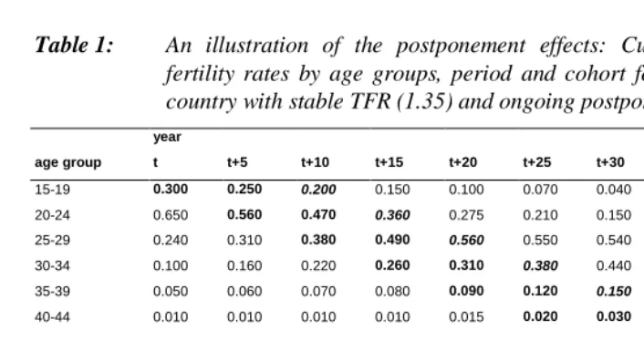
2.5. Timing effects in period fertility: An illustration
the TFR below 2.10). The ‘lowest-low fertility’ is typically associated with a marked postponement of childbearing. Therefore, it is a temporary phenomenon which does not lead to the similarly (lowest-)low cohort fertility6. Table 1 provides an illustration of this situation. Suppose that a country experiences a transition from early to late childbearing. This transition takes 35 years, during which the mean age of fertility schedule (MAB) increases every year by 0.2 years of age.
Table 1: An illustration of the postponement effects: Cumulative age-specific
fertility rates by age groups, period and cohort fertility indicators in a country with stable TFR (1.35) and ongoing postponement of births
year
age group t t+5 t+10 t+15 t+20 t+25 t+30 t+35 index (t+35)/t 15-19 0.300 0.250 0.200 0.150 0.100 0.070 0.040 0.020 0.07
20-24 0.650 0.560 0.470 0.360 0.275 0.210 0.150 0.110 0.17
25-29 0.240 0.310 0.380 0.490 0.560 0.550 0.540 0.480 2.00
30-34 0.100 0.160 0.220 0.260 0.310 0.380 0.440 0.500 5.00
35-39 0.050 0.060 0.070 0.080 0.090 0.120 0.150 0.200 4.00
40-44 0.010 0.010 0.010 0.010 0.015 0.020 0.030 0.040 4.00
TFR 1.350 1.350 1.350 1.350 1.350 1.350 1.350 1.350 MAB 23.72 24.72 25.72 26.72 27.72 28.72 29.72 30.72 Change in MAB 1.00 1.00 1.00 1.00 1.00 1.00 1.00
Cohort 1 1.610 Cohort 2 1.670 Cohort 3 1.690
Over the whole period, the TFR remains at a low level of 1.35. One might expect a decline in the cohort fertility towards the level of the period TFR over such a long period and, more generally, the convergence between the cohort and period TFR.
countries over the 1990s. Fertility schedule in the year t resembles the schedule in Bulgaria in 1994 (TFR=1.37, MAB =24.1 years), the schedule in the year t+10 comes close to the schedule in Romania in 1998 (TFR=1.32, MAB=25.4 years), the schedule in the year t+25 resembles the situation in Spain in 1990 (TFR=1.36, MAB=28.9 years) and the schedule in the year t+35 has a similar profile as the fertility schedule in the Netherlands in 1999 (though the TFR of 1.65 was considerably higher there; MAB=30.3). While the tempo effects are now commonly recognised as a source of temporal variations in the TFR, many researchers assume that such influences are relatively short-lived. This illustration has shown that the TFR may give misleading signals about the trends in cohort fertility over a long period of time.
3. Methods
3.1. Linking period and cohort fertility
The core of the analysis lies in the comparison of period and cohort fertility indicators. The period indicators in a particular year are compared with the values of completed
cohort fertility of women who reached the mean age at childbearing7 in that year.
Similarly, figures depicting period and cohort fertility trends display cohort indicators shifted by the period mean age at childbearing to enable a straightforward comparison of the period and cohort values. In other words, period and cohort indicators are linked in the following way:
Let Y be year of birth of a generation of women whose completed cohort fertility of parity i is compared with the period fertility of birth order i in calendar year t. Then
Y = t – MABi (1)
where MABi is mean age of fertility schedule computed from age-specific fertility rates (ASFR) of birth order i in the year t. Y is then rounded down or up to the nearest whole number.
å
å
åå
å
+
=
=
=
i i a
F t a
t i a
a
t i a i
t i t
P
B
ASFR
TFR
TFR
5 . 0 ,
, , ,
, ,
high ages. The potential fertility ‘catch-up’ is likely to be small in the late ages of childbearing and therefore no specific assumptions have been made.
Differences between period and cohort indicators are compared separately for each birth order (see Section 6). The indicators were computed for all birth orders specified in the source data, with the last category including all the subsequent birth orders (see Table 2). Taking into account the very small share of high birth orders on total fertility, the indicators for birth order 3 and higher were combined for comparative analysis. The average values of annual absolute difference between the period TFR and the ultimate cohort fertility serve as a benchmark, establishing how closer other period fertility indicators approximate the CFR. Visual inspection of figures comparing the trends of various fertility indicators adds another dimension to the judgement of their ‘performance’ over time. Selected additional criteria, such as fluctuations in the period fertility measures, the occurrence of ‘impossible’ values, the performance in ‘extreme situations’ and the analysis of period-cohort fertility differences in the periods of rapid postponement are discussed in Section 7.
3.2. Indicators of period fertility used in the analysis
Following indicators of period fertility are compared in the analysis:
1. Total fertility rates (TFRi) by birth order i, computed as a sum of reduced age and order-specific fertility rates (ASFRi). The TFR is a sum of order-specific TFRi :
(2)
where a is age, t calendar year (t+0.5 stands for the mid-year population), B number of live births, P population size and F denotes females.
2. The ‘tempo-adjusted’ order-specific total fertility rates (adjTFRi) proposed by Bongaarts and Feeney are calculated as follows:
adjTFRi,t = TFRi,t / (1-ri,t) (3)
F t i a t i a t i
a
B
P
q
,,=
,, ,−1,ri,t =(MABi,t+1 – MABi,t-1) / 2 (4)
where MABi,t is the mean age of fertility schedule of order i, calculated from reduced rates (ASFRi,t). This computation is followed in the analysis. Alternatively, as suggested by Zeng Yi and Land (2001: 19, fn. 7), change in median age may be calculated. Although they found median age less sensitive to random fluctuations, in the case of the four countries analysed in this paper change in the median age displayed on average slightly wider fluctuations than the change in the mean age, particularly in the case of Sweden in 1990-1993.
Analogous to the TFR (see eq. 2), the tempo-adjusted total fertility rate for all birth orders is computed as a sum of the adjusted order-specific total fertility rates.
3. Period fertility indicator derived from the parity-specific birth probabilities (PATFRi).
Age-specific and parity-specific birth probabilities qa,i serve as an input of the multistate (increment-decrement) fertility table, treating each birth order separately (for the classification of life tables see Willekens, 1991). Following Rallu and Toulemon (1994: 66), birth probabilities are estimated directly from the data on births and parity and age structure of women:
(5)
Thus, Equation 5 expresses the probability that a woman aged a and having i-1 children will give birth during the year t. Different from the ASFRa,i,t calculation in Equation 2, the denominator is the parity-specific female population at the beginning of the year t.
Here, an illustration of the fertility table computation is provided for parity 1. Consider a population of 10,000 women entering fertility table of parity 1 at age 12:
All women are initially childless. The apostrophe distinguishes table population P’ from
the real population P. Number of women still remaining childless at age x (x≥13) is
given as (see Rallu and Toulemon, 1994: 66, Eq. 2):
(6)
000
,
10
'
12,0,=
F t
P
(
)
∏
< ≤−
=
x y y F Fx
P
q
P
12 1 , 0 , 12 0,
'
1
F F
F F
F
i
P
P
P
P
P
PATFR
1=
'
50,≥1/
'
12,0=
(
'
12,0−
'
50,0)
/
'
12,0and number of ultimately childless women is equal to the table number of childless women at age 50 (P’F50,0). The first parity index of total fertility (PATFR1) is computed as a proportion of women who had at least one child during their reproductive life (ages 12 and 50 are considered here as limits for reproduction):
(7)
If, for instance, 1,000 women out of the initial 10,000 were to remain childless at age
50, the PATFR1 would be (10,000-1,000) / 10,000 = 0.90, i.e. 90% of women in the
table population would ultimately have at least one child.
Women having their first child at age a leave the fertility table of first births and enter the table of parity 2, that is they become exposed to the probability of having a second birth since the age a+1. In a similar way as for the first parity, the PATFR of parity 2 may be calculated as the table number of women who have at least two children divided by the initial number of childless women:
(8)
Parity progression ratios, probabilities of having another child by age and current parity and a number of other indicators can be computed from these sequential fertility tables (see Ortega and Kohler, 2002). Tables of fertility also provide the synthetic (table) parity distribution of women by age, given birth probabilities of a selected year or period.
Fertility tables for the highest parity category, denoted as U (4+ in Italy, the Netherlands and Sweden; 5+ in the Czech Republic), were estimated as an open-ended category, depicting the probability of having another birth among women with at least U-1 children:
(9)
4. Tempo-adjusted and variance-adjusted period fertility indicator derived from the parity-specific birth probabilities (adjPATFRi)
Kohler and Ortega (2002a) proposed an indicator derived from birth probabilities that provides adjustment both for the tempo and variance effects. Their method enables an estimation of the period fertility measures that are free of the three distortions present in the TFR, namely distortions caused by (1) changes in the parity distribution of women, (2) changes in fertility timing and (3) changes in the variance of fertility schedule. It is an analogy of the method developed earlier by Kohler and Philipov (2001) for an adjustment of the reduced period fertility rates (see also Section 2.2). The
F F
F F F
F
i
P
P
P
P
P
P
PATFR
2=
'
50,≥2/
'
12,0=
(
'
12,0−
'
50,0−
'
50,1)
/
'
12,00
;
/
, 1,, , ,
,≥
=
B
≥P
≥ −U
>
authors employ a procedure that iteratively corrects the observed mean age and the inferred tempo for distortions caused by the variance effects (Kohler and Philipov, 2001: 10). They recommend smoothing the observed probabilities before using this method. While using unsmoothed probabilities, only a rough adjustment of birth
probabilities for variance effects is provided in this paper8. Parity-specific tempo
change ra,i,t was computed following Kohler and Philipov (2001: 8, Eq. 11):
ra,i,t = γi,t + δa-a*,i,t (10)
where γi,t is the annual change in the mean age of birth probability schedule of parity i, δ is the annual increase in the standard deviation of the schedule and a* is the mean age of probability schedule. Indicator γi,t was estimated from the mean age of probability
schedule in a similar manner as the Bongaarts-Feeney estimate of ri,t in Equation 4
above. Estimation of δ was based directly on an estimate in Result 12 in Kohler and
Philipov (2001: 10), without performing the iterative procedure described in Result 13.
4. Data
Period and cohort fertility data were obtained from various sources listed in Appendix 1. Table 2 provides for each country an overview of the primary data and derived reduced rates and birth probabilities by birth order and age. It further shows for which periods various summary indicators were estimated.
Time series of reduced rates generally cover longer periods of time than the series of birth probabilities. Birth probabilities were computed directly from the data on births by birth order and age of mother and age and parity structure of women, following Equation 5 above. All births were organised in the period-cohort perspective. In the case of the initial data organised in the age-period perspective, a simple linear approximation was used to estimate the structure of births in the period-cohort manner:
Ba,i,t = (BA-1,i,t + BA,i,t) / 2 (11)
where a is age reached during the year t (cohort age) and A is age in completed years at the time of birth B.
These time series were obtained by combining the initial cumulative cohort fertility distribution and period reduced rates prior and after the year for which it was available. This method assumes that migration and mortality do not affect cohort fertility, that is the distribution by the number of children in each birth cohort is the same among women who die or migrate and women who survive and stay in the country. Although foreign-born women frequently have a different number of children than their native counterparts, this does not have a large influence on the reconstruction of cohort fertility for a relatively short period of time, particularly in countries with fairly low immigration, such as Italy and the Czech Republic. An overview of the reconstructed cohort fertility data is provided in Table 2; a detailed description of data sources and estimates of cohort fertility is given in Appendix 1.
Table 2: Overview of period and cohort fertility data used in the analysis
Czech Republic Italy The Netherlands Sweden Primary data Ba,i, PFa Ba,i PFa (1980-85, 1990-97) Ba,i, PFa Ba,i PFa
ASFR (1965-79, 1985-89)
Observation perspective AP AP (PC in 1991-97) PC PC Birth order 1-5+ 1-5+ (1-4+ in 1965-79 and 85-89) 1-4+ 1-5+ Derived measures:
ASFRi, TFRi 1966-2000 1965-1997 1965-2001 1975-2000
AdjTFRi 1966-1999 1965-1996 1965-2000 1975-1999
Birth probabilities qa,i and PATFRi 1966-2000 1980-1997 1980-2001 1980-2000
AdjPATFRi 1966-1999 1981-1996 1981-2000 1981-1999
'Corresponding' completed cohort fertility indicators are compared with period fertility measures for a given period: 1966-1992 1965-1989 1965-1994 1975-1993 Cohort CFR C1916-1987 C1933-1983 C1930-1987 C1930-1986 Period for which CFR estimated 1) 1965-2001 1980-1998 1980-2002 1980-2001 Notes:
1) Period for which cumulative cohort fertility by parity is reconstructed for all women of reproductive age. Observation perspective: AP age-period perspective (births organised by the exact age of mother)
PC period-cohort perspective (births organised by the year of birth of mother) See Appendix 4 for an overview of symbols for various fertility indicators.
5. Four countries, four fertility histories
Four countries, roughly representing four European regions – Western Europe (the Netherlands), Northern Europe (Sweden), Southern Europe (Italy) and Central-Eastern Europe (the Czech Republic) – also constitute examples of four different fertility histories.
decade of rapid fertility decline (1965-1975) replaced by fairly stable low-fertility values (TFR below 1.65 between 1976 and 1998), influenced by the ongoing postponement of births. The increase in period fertility after 1995 was connected with a slow-down of the fertility postponement (Figure 2). The TFR value of 1.72, reached in 2000, was the highest since 1974.
In Sweden, the total fertility rate declined after the moderate baby boom in the mid-1960s, in line with trends in Italy and the Netherlands. However, since 1986 Sweden experienced a distinct baby-boom period culminating in 1990 (TFR 2.13). This fertility swing, quite unusual in the countries of the European Union after the 1960s, was partly induced by an extension of the period of eligibility to paid parental leave for mothers in 1986. This measure has ‘speeded up’ the births of second and later children (Sundström and Staffoerd, 1992; Andersson, 1999; Hoem and Hoem, 2000).
Figure 1a: TFR in the Czech Republic, Italy, the Netherlands and Sweden, 1960-2000
Figure 1b: Completed fertility of female birth cohorts in the Czech Republic, Italy, the Netherlands and Sweden
1.00 1.50 2.00 2.50 3.00 3.50
1960 1965 1970 1975 1980 1985 1990 1995 2000 Year
TFR
Czech Republic Italy The Netherlands Sweden
1.00 1.20 1.40 1.60 1.80 2.00 2.20 2.40 2.60 2.80
1925 1930 1935 1940 1945 1950 1955 1960 1965 Birth cohort
CF
R
Cohort fertility in these countries was characterised by a considerable stability as the ups and downs of period fertility have affected cohort values to a much smaller degree (Figure 1b). Cohort fertility of women in Sweden and the Czech Republic depicted a stable level around or somewhat above 2.0 children per women up to the cohorts born in the early 1960s. Cohort fertility of Dutch and Italian women was gradually decreasing, more rapidly (and from higher levels) among Dutch women born in the 1930s and in the 1940s and among Italian women born in the 1950s. Cohorts of women born around 1945 had on average around 2 children in all four countries (between 1.95 in the Netherlands and 2.06 in Italy). Among younger cohorts, however, the differences have increased again: in Italy and Sweden women born in 1960 have on average less than 1.7 children and 2.05 children, respectively.
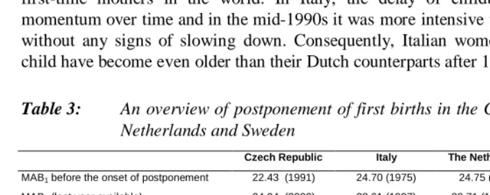
Table 3 and Figure 2 provide an overview of the extent of postponement of first births, as captured by the increase in the period mean age of first-time mothers. The delay in first births had started earlier than in subsequent births and it has had the strongest impact on the total fertility rates. In Italy, the postponement started in 1975 – by several years later than in Sweden and the Netherlands. Since then, the mean age of first-time mothers has increased by almost 4 years in these countries. It is only in the Netherlands that the increase has, at least temporarily, come to an end in 1999. Until then, the Netherlands had been a ‘champion’ of delayed motherhood, having the oldest first-time mothers in the world. In Italy, the delay of childbearing was gaining momentum over time and in the mid-1990s it was more intensive than ever before, still without any signs of slowing down. Consequently, Italian women bearing their first child have become even older than their Dutch counterparts after 1997.
Table 3: An overview of postponement of first births in the Czech Republic, Italy,
Netherlands and Sweden
Czech Republic Italy The Netherlands Sweden MAB1 before the onset of postponement 22.43 (1991) 24.70 (1975) 24.75 (1971) <24.21 (1974) b)
MAB1 (last year available) 24.94 (2000) 28.61 (1997) 28.71 (1998) a) 27.87
Duration of the postponement, years 9 22 27 26+ Total increase in MAB1, years 2.51 3.91 3.96 3.66
Average annual increase in the MAB1 0.28 0.18 0.15 0.14
Average annual change in the MAB1 during the following periods:
1970-1975 0.01 -0.08 0.08 ..
1975-1980 -0.03 0.08 0.11 0.16
1980-1990 0.01 0.17 0.19 0.10
1990-1995 0.17 0.22 0.17 0.17
1995-2000 0.32 0.39 (95-97) 0.04 0.14
MAB1 Mean of mother at birth of first child (computed from the age-specific reduced rates)
Notes: a) in 1999, the MAB1 declined for the first time since 1971
Figure 2: Mean age of mother at birth of first child in the Czech Republic, Italy, the Netherlands and in Sweden, 1960-2000
In the Czech Republic postponement has started much later, in 1992. By that time, Czech women were bearing children at an early age, in line with the pattern in other post-communist countries of Europe. Since then postponement of first births has been proceeding much faster there than in the other three countries under discussion. Due to the initially very young age at childbearing, a large scope for further delay still exists in the Czech Republic: by 1999, the mean age of women at birth of their first child has reached the levels recorded in the Netherlands, Sweden and Italy in the early 1970s.
6. Comparison of period and cohort fertility by birth order
6.1. Fertility of birth order 1
More intensive and longer-lasting postponement has ‘deflated’ period total fertility of first birth order more than fertility at higher orders. Therefore, we could expect that fertility measures adjusted for the tempo changes differ from the TFR especially in the case of order 1.
20.0 22.0 24.0 26.0 28.0 30.0
1960 1965 1970 1975 1980 1985 1990 1995 2000 Year
MA
B
1
Figure 3: Period and cohort fertility indicators of birth order 1 in the Czech Republic, Italy, the Netherlands and Sweden
0.50 0.60 0.70 0.80 0.90 1.00 1.10 19 65 19 70 19 75 19 80 19 85 19 90 19 95 20 00 TFR adjTFR PATFR adjPATFR CFR1 Czech Republic 0.50 0.60 0.70 0.80 0.90 1.00 1.10 196 5 197 0 197 5 198 0 198 5 199 0 199 5 200 0 TFR adjTFR PATFR adjPATFR CFR1 The Netherlands 0.50 0.60 0.70 0.80 0.90 1.00 1.10 196 5 197 0 197 5 198 0 198 5 199 0 199 5 TFR adjTFR PATFR adjPATFR CFR1 Italy 0.50 0.60 0.70 0.80 0.90 1.00 1.10
1975 1980 1985 1990 1995 2000
Country-specific results are depicted in Appendix 3. All analysed alternative indicators provide better approximation of cohort fertility than the TFR1. Only in the case of the
Czech Republic, the Bongaarts-Feeney adjTFR did not provide closer approximation of the cohort CFR. During most of the analysed period (1966-1992), the timing of first births was very stable there and the tempo effects were absent. It is worth mentioning that under these conditions the PATFR indicators derived from the fertility table of first births showed considerably higher stability than the TFR and displayed only a negligible difference from the cohort CFR (see Figure 3). The period around 1975 is of particular interest. Following the recently implemented family policy measures, period
indicators increased considerably (TFR1 was above the level of 1.0 in 1974-1976),
coinciding with a short-time advancement of first births. For this period (see Table A in Appendix 3), indicators based on probabilities show that most of the increase in the
TFR1 was due to the timing changes and distortions in the distribution of women by
parity. The PATFR1 as well as the adjusted adjPATFR1 show stable values of 0.94-0.95, corresponding closely to the final cohort fertility of parity 1.
During the strong timing-shifts, characterised by the highest differences between
the period TFR1 and the cohort CFR1, all alternative indicators came considerably
closer to the CFR1. They particularly show different values of period fertility in the
Czech Republic during the second half of the 1990s when the TFR1 declined to an
extreme level of 0.52-0.539. Fertility table indicator adjPATFR1 for the same period
reached levels of 0.85-0.93 (see Appendix 2), which do not imply a dramatic increase in cohort childlessness in the future.
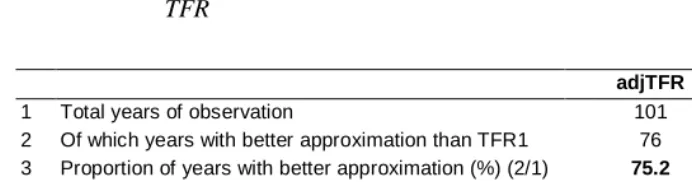
Table 4 summarises the performance of fertility indicators of birth order 1 for all countries combined. The indicators based on probabilities, the PATFR and particularly
its adjusted version provide the closest approximation of the cohort CFR1. The
adjPATFR comes closer to the cohort fertility in 81% of the cases (non-adjusted PATFR
even in 89% of the cases) and it reduces on average the difference between TFR1 and
Table 4: Summary table for birth order 1. Degree to which the period fertility indicators approximate completed cohort fertility in comparison with the TFR
adjTFR PATFR adjPATFR
1 Total years of observation 101 63 63 2 Of which years with better approximation than TFR1 76 56 51 3 Proportion of years with better approximation (%) (2/1) 75.2 88.9 81.0
Average absolute differences from completed cohort fertility values
4 Average abs. difference of TFR1 (%) 10.68 10.55 10.55 5 Average abs. difference of alternative measure (%) 5.44 3.31 2.52 6 INDEX (4-5)/4 (index of improvement in approximation) 0.49 0.69 0.76
Figure 3 displays period and cohort fertility in each country. It amply illustrates the advantages and disadvantages of the use of particular period measures. The adjusted adjTFR usually displays values closer to the CFR than the ordinary TFR. However, it also shows considerable fluctuations with ups and downs that are difficult to interpret. It can also reach ‘impossible’ values of first-order TFR over 1.0, for instance in Sweden in 1975 and in 1990-1993 (see Section 7.3). The indicators based on birth probabilities are more stable and, by definition, remain within the theoretically possible range of cohort fertility distributions. The PATFR shows high stability and very good correspondence with the cohort fertility in the periods with no changes in fertility timing, such as in the Czech Republic before 1992. On the other hand, it displays systematically lower values than the corresponding cohort CFR during the periods of
the postponement. Adjusted adjPATFR1 comes close to the ultimate cohort fertility in
most cases shown in the graphs and approximates the CFR1 particularly well in the case
6.2. Fertility of birth order 2
In most cases, the Bongaarts-Feeney adjTFR approximated values of the completed cohort fertility of birth order 2 better than the TFR2 indicators, particularly in the case of
Italy, where the change in the TFR2 as well as in the mean age at childbearing was
without sudden fluctuations (see Table B in Appendix 3). However, there were
considerable fluctuations in the adjTFR in the Czech Republic (in the second half of the 1960s and around 1993) and in Sweden (around 1994), which again should lead to due care in interpreting this indicator in terms of the cohort fertility expectations. The use of the PATFR for an approximation of the cohort fertility of second parity is not justified. It does not come considerably closer to the cohort fertility than the period indicators of
the TFR2 (the average ‘improvement’ in approximation is only by 25%; see Table 5).
Clearly, the timing effects influence the fertility table measures of second births in a similar way as they affect the period TFR. The summary PATFR indicator for parity 2 provided good results only for the Czech Republic in the 1970s and 1980s, that is in the period unaffected by larger shifts in fertility timing.
Though the table indicators are more elaborate than the measures based on reduced rates, they do not lead to a closer approximation of cohort fertility of parity 2 than the
relatively simple Bongaarts-Feeney adjustment of the TFR. The adjPATFR2
Figure 4: Period and cohort fertility indicators of birth order 2 in the Czech Republic, Italy, the Netherlands and Sweden
0.40 0.60 0.80 1.00
1
965 1970 1975 1980 1985 1990 1995 2000 TFR adjTFR PATFR adjPATFR CFR2 Czech Republic 0.40 0.60 0.80 1.00 1
965 1970 1975 1980 1985 1990 1995 2000
Table 5: Summary table for birth order 2. Degree to which the period fertility indicators approximate completed cohort fertility in comparison with the TFR
adjTFR PATFR adjPATFR
1 Total years of observation 101 63 63 2 Of which years with better approximation than TFR2 74 50 50 3 Proportion of years with better approximation (%) (2/1) 73.3 79.4 79.4
Average absolute differences from completed cohort fertility values
4 Average abs. difference of TFR2 (%) 11.02 12.28 12.28 5 Average abs. difference of alternative measure (%) 4.93 9.19 5.91 6 INDEX (4-5)/4 (index of improvement in approximation) 0.55 0.25 0.52
6.3. Fertility of birth order 3 and higher
The alternative period fertility indicators do not improve the approximation of completed cohort fertility of birth order 3 and higher. The fertility table indicator (PATFR3+) even gives considerably worse results than the period TFR3+ in all compared
situations (Table C in Appendix 3, Table 6 and Figure 5). The adjusted adjPATFR3+
eliminates part of the differences between the PATFR3+ and the cohort CFR3+.
However, it still provides poorer approximation of cohort fertility than the ordinary TFR3+.
Out of all considered indicators, only the Bongaarts-Feeney adjTFR3+ provides a
slightly better approximation of the cohort CFR3+. Still, the improvement is very
modest: although it comes closer to the CFR3+ in 77% cases as compared with the
TFR3+, it reduces the difference on average only by 23%.
Table 6: Summary table for birth order 3+. Degree to which the period fertility
indicators approximate completed cohort fertility in comparison with the TFR
adjTFR PATFR adjPATFR
1 Total years of observation 101 63 63 2 Of which years with better approximation than TFR3+ 71 8 17 3 Proportion of years with better approximation (%)
(2/1)
70.3 12.7 27.0
Average absolute differences from completed cohort fertility values
4 Average abs. difference of TFR3+ (%) 11.99 11.51 11.51 5 Average abs. difference of alternative measure (%) 9.24 28.11 22.18 6 INDEX (4-5)/4 (index of improvement in
approximation)
Figure 5: Period and cohort fertility indicators of birth order 3+ in the Czech Republic, Italy, the Netherlands and Sweden
0.00 0.10 0.20 0.30 0.40 0.50 196 5 197 0 197 5 198 0 198 5 199 0 199 5 200 0 adjTFR PATFR adjPATFR CFR3+ 0.00 0.20 0.40 0.60 0.80 1.00 1.20
1965 1970 1975
0.20 0.25 0.30 0.35 0.40 0.45 0.50 19 75 19 80 19 85 19 90 19 95 20 00 TFR adjTFR PATFR adjPATFR CFR3+ The Netherlands 0.00 0.10 0.20 0.30 0.40 0.50 0.60 0.70 0.80 0.90
1965 1970 1975
0.00 0.10 0.20 0.30 0.40 0.50 0.60
1975 1980 1985 1990 1995
Thus, also the performance of the adjTFR for birth order 3+ is considerably worse than for the lower orders. Relatively slower postponement of third and later births (as compared with first and second births) as well as random fluctuations in the mean and median age of mother at third and higher birth orders influenced negatively the performance of the Bongaarts-Feeney adjustment. As a result, none of the alternative period fertility measures is suitable even for a rough approximation of higher-parity cohort fertility. This issue is further addressed in Section 8.
6.4. All births combined: Period indicators of total fertility
Table D in Appendix 3, Table 7 and Figure 6 provide an overview of the approximation of cohort fertility using different indicators of period fertility for all birth orders. One additional indicator is introduced here. A hybrid indicator (comTFR), which combines the adjPATFR indicator for parity 1 and 2 with the TFR for birth order 3+. The rationale was to combine indicators that approximate best the cohort fertility at each birth order. For birth order 3 and higher, the TFR was chosen instead of the adjTFR due to the large year-to-year fluctuations in the latter measure.
Table 7: Summary table for indicators of total fertility. Degree to which the period fertility indicators approximate completed cohort fertility in comparison with the TFR
adjTFR PATFR adjPATFR comTFR
1 Total years of observation 101 63 63 63 2 Of which years with better approximation than TFR 83 47 50 53 3 Proportion of years with better approximation (%) (2/1) 82.2 74.6 79.4 84.1
Average absolute differences from completed cohort fertility values
4 Average abs. difference of TFR (%) 12.09 10.81 10.81 10.81 5 Average abs. difference of alternative measure (%) 6.56 9.10 6.24 4.15 6 INDEX (4-5)/4 (index of improvement in approximation) 0.46 0.16 0.42 0.62
The evidence provided by the order-specific comparison of period and cohort fertility indicators may be summarised as follows:
(i) Various indicators of period fertility provide different results, and therefore often imply contradictory interpretations of fertility trends. Differences between the indicators induced by period effects are heterogeneous with respect to birth order. For instance, during the periods of increasing mean age at childbearing the PATFR consistently displays higher fertility than the TFR at birth order 1, but at the same time it shows considerably lower levels of fertility at higher parities (3+).
(ii) All period indicators fluctuate more than the relatively stable cohort fertility rate. This is consistent with the fact that period measures reflect period influences that are often temporary and less stable than the cohort trends, which we may think of as an aggregate result of changes over a long period of time. Some period fluctuations may be interpreted in terms of plausible explanations (population policy measures, economic influences etc.), yet others seem to be artificial results of applying a particular adjustment method or using particular indicators of period fertility. The issue of fluctuation in fertility indicators is further addressed in Section 7.2.
Figure 6 Period and cohort fertility indicators (all parities) in the Czech Republic, Italy, the Netherlands and Sweden
1.00 1.25 1.50 1.75 2.00 2.25 2.50
1965 1970 1975 1980 1985 1990 1995 2000
TFR adjTFR PATFR adjPATFR comTFR CFR Czech Republic
1.00 1.50 2.00 2.50 3.00
1965 1970 1975 1980 1985 1990 1995 2000
TFR adjTFR PATFR adjPATFR comTFR CFR The Netherlands
1.00 1.50 2.00 2.50 3.00
1965 1970 1975 1980 1985 1990 1995
TFR adjTFR PATFR adjPATFR comTFR CFR Italy
1.00 1.20 1.40 1.60 1.80 2.00 2.20 2.40
1
975 1980 1985 1990 1995 2000
7. Additional criteria to analyse the performance of period fertility
indicators
7.1. Approximation of cohort fertility in periods of intensive postponement
So far the paper has discussed the period-cohort fertility differences in various situations, including periods with no important changes in fertility timing. However, the main issue of the adjustment is an estimation of fertility quantum in periods when the TFR is influenced by the tempo shifts in childbearing. A brief additional analysis focuses on the periods in which the mean age at first birth increased by at least 0.1 years in a calendar year and for which all compared indicators were estimated. This illustration comprises the evidence for 26 calendar years: for the Netherlands between 1981 and 1993, for Italy between 1981 and 1989 and for Sweden between 1981 and 1984.
The summary table (Table 8) suggests that the period indicators other than the TFR indeed reduce the difference between the TFR and the completed cohort fertility especially in the periods marked by a postponement of childbearing. All indicators in the table came closer to the CFR in all the years of observation. While the PATFR reduced the TFR-CFR difference only by a margin, the remaining indicators reduced this difference on average by more than 60%, the adjTFR by 74% and the comTFR even by 77%. The average difference between the TFR and the CFR, which was 17.1%, has shrunk to only 4.0% distance between the comTFR and the CFR.
If these findings reflect reality – and we would need more observations to draw such a conclusion – then several period indicators provide considerably better approximation of cohort fertility during the shifts in the timing of births and thus indicate to a large extent the ‘underlying’ levels in cohort fertility and better reflect the period quantum.
Table 8: Summary table of the performance of different period fertility indicators: Degree to which they approximate completed cohort fertility during an intensive postponement of first births
adjTFR PATFR adjPATFR comTFR
Total years of observation 26 26 26 26 Of which years with better approximation
than TFR
26 26 26 26
Proportion of years with better approximation (%) (2/1)
100 100 100 100
Average absolute differences from completed cohort fertility values
Average abs. difference of TFR (%) 17.13 17.13 17.13 17.13 Average abs. difference of alternative
measure (%)
4.53 14.80 6.45 4.02
INDEX (4-5)/4 (index of improvement in approximation)
0.74 0.14 0.62 0.77
In sum, adjusted indicators do not seem to provide too optimistic (read: high) approximation of cohort fertility. Moreover, smoothing or averaging values for longer periods erases some random fluctuations and thus further reduces the period-cohort fertility differences.
Table 9: Average relative differences between period fertility indicators and the
corresponding final cohort fertility (CFR) over longer periods of time (in %)
The Netherlands Italy Sweden Total
Period 1981-1993 1981-1989 1981-1984
Years of observation 13 9 4 26
TFR -15.3 -18.7 -19.6 -17.1
AdjTFR 1.8 -2.0 -7.3 -0.9
PATFR -13.5 -15.2 -18.2 -14.8 AdjPATFR 0.1 -5.5 -10.8 -3.5
7.2. Fluctuations in fertility indicators
Period fertility indicators are characterised by less stability than the cohort fertility rates. If one source of instability, the tempo component, is removed, these indicators may be expected to reflect higher stability and fewer fluctuations. However, previous sections have shown that the adjusted indicators are often less stable than the total fertility rates. This instability seems to reflect random fluctuations, which can not be explained by any underlying causes.
To look at these fluctuations in a more systematic way, the average annual absolute change in all the considered indicators was analysed. Table 10 shows the average annual fluctuations as well as relative fluctuations with respect to the TFR and CFR. It depicts substantial differences by birth order. Period indicators are characterised by considerably more intensive annual changes than the cohort CFR. The most stable period indicator of order 1 and 2 is the PATFR and for total fertility it is the combined indicator comTFR. The adjusted adjPATFR is more stable than the TFR for order 1 and roughly as stable as the TFR for order 2. However, for birth order 3 and higher, all indicators based on birth probabilities are much more volatile than the TFR. The adjTFR is almost as stable as the TFR for birth orders 3+ and for all orders combined, while in the case of birth order 1 it depicts higher fluctuations. In general, we may suspect indicators that are more volatile than the TFR – the adjTFR for parity 1 and the PATFR and adjPATFR for parity 3 and higher – to be subjected to the strongest random fluctuations.
Table 10: Average absolute annual changes in fertility indicators by birth order.
Summary of data for 59 years (Czech Republic 1967-92, Italy 1982-89, the Netherlands 1982-94, Sweden 1982-93)
Average annual change in a given indicator (%)
TFR adjTFR PATFR adjPATFR comTFR C FR All parities 2.67 2.79 2.21 3.14 1.98 0.66 Parity 1 2.31 3.69 0.71 1.35 .. 0.36 Parity 2 3.06 3.43 2.17 3.15 .. 0.63 Parity 3+ 3.06 3.43 7.28 11.16 .. 1.91
Changes relative to the TFR (Average fluctuations in TFR = 1.0)
All parities 1.00 1.04 0.83 1.18 0.74 0.25 Parity 1 1.00 1.60 0.31 0.58 .. 0.16 Parity 2 1.00 1.12 0.71 1.03 .. 0.21 Parity 3+ 1.00 1.12 2.38 3.64 .. 0.62
Changes relative to the CFR (Average fluctuations in CFR = 1.0)
7.3. ‘Impossible’ cases
It is a well known fact that the TFR may reach levels that can not occur in the real birth cohorts, such as the first-order TFR higher than 1.0, suggesting an absurd situation of more than 100% of women in a synthetic cohort having their first child. Such cases do not occur in multiplicative measures, where women are not exposed to a birth of certain parity more than once. Impossible values depicted occasionally by the TFR may still be acceptable as indicators of the short-time trends in period fertility, but they point out how limited the TFR is for any approximations of cohort fertility or assessments concerning the consequences of ‘current’ fertility rates.
From the total of 127 observations, the TFR1 exceeded the level of 1.0 in 6 cases
(4.7%) – in the Czech Republic in 1974-75, in the Netherlands in 1965-67 and in Italy
in 1965. The adjusted TFR1 was in all these cases below 1.0, indicating that the TFR
was ‘exaggerated’ due to the tempo effects, namely due to the advancement of births. On the other hand, the adjTFR1 exceeded unity in 7 other cases: in Sweden in 1975 and
in 1990-1993 and in the Czech Republic in 1971 and 1994. Apparently, the tempo-adjusted TFR can not be used for the projections of cohort fertility trends unless extreme caution is exercised.
7.4. Performance in ‘extreme’ situations
Zeng Yi and Land (2001: 23) concluded in their sensitivity analysis of the Bongaarts-Feeney adjTFR that the formula “often is not sensitive to its underlying assumption about the invariant shape of the fertility schedules and equal changes in timing across ages” and “usually does not differ from an adjusted TFR(t), which allows the shape of the fertility schedule to change at a constant annual rate”. This simplifying assumption was one of the major points of criticism against the use of the Bongaarts-Feeney approach (see Van Imhoff and Keilman, 2000; Kohler and Philipov, 2001 and Van Imhoff, 2001). However, according to Zeng Yi and Land, ‘extremely large’ changes in the fertility tempo and in the shape of the fertility schedule may distort the performance of the BF adjustment. Changes in the mean age of fertility schedule exceeding 0.25 years per calendar year, particularly when coupled with the changes in the interquartile range of fertility schedule exceeding 0.10 years were suggested to be such instances (Zeng Yi and Land, 2001: 23).
countries with an intensive postponement of births in the 1990s, particularly Italy and the Czech Republic. Especially the Czech Republic after 1993 is a model case of ‘extreme’ situations: the mean age of fertility schedule at first birth has been increasing by an annual rate of 0.24-0.41 years and the interquartile range by 0.09-0.30 years, slowing down only in 2000.
The Bongaarts-Feeney adjustment of first-order fertility in the Czech Republic (adjTFR1, see Figure 3 and Appendix 2) does not – with the exception of a brief upward
fluctuation in 1992-1994 – seem to show exaggerated valuesas would be suggested by
Zeng Yi and Land’s (2001) findings. Generally, during the periods of rapid increase in the mean age or intensive changes in the interquartile range adjusted indicators do not show stronger fluctuations or larger differences from cohort fertility. Many fluctuations appear to occur because of random influences or nonsystematic changes, such as large and time-varying changes in the tempo and shape of the schedule (Zeng Yi and Land, 2001: 23). This applies also for the adjustment for variance effects, which often generates additional fluctuations10.
7.5. Calculating period fertility indicators
There are two major sources of difficulties in the calculation of the ‘alternative’ period fertility indicators. Firstly, not all the necessary data are available. Secondly, calculation of some measures is much easier than the derivation of other indicators. Larger data availability and easier computation potentially contribute to a wider acceptance and more extensive use of analysed indicators.
In almost all European countries data on births by age of mother, necessary for computing the TFR, are available. Nevertheless, some countries (Belgium, France until 1996, Germany, United Kingdom and Switzerland) collect and publish data on birth order within the current marriage, which is not a reliable indicator of birth distribution in countries with a high proportion of non-marital births. The use of such data for calculating order-specific indicators should be avoided. In some cases, e.g. in the United Kingdom, large national surveys enable detailed estimates of age and order-specific fertility indicators (see Smallwood, 2002b). The calculation of birth probabilities requires data on births by age of woman and parity as well as the composition of the female population by parity. This is often not available, particularly for the ‘true’ (biological) birth order. Cohort indicators may be estimated on the basis of period data; nevertheless, time series covering sufficiently long periods of time are usually unavailable.
calculation of tempo and variance-adjusted measures, proposed by Kohler and Philipov (2001) and Kohler and Ortega (2002a), involves an elaborate procedure. It is therefore very likely that the latter indicators will not become widespread and generally recognised alternatives to the TFR.
8. Discussion on the tempo-quantum and period-cohort interaction
Why are there such large differences by birth order in the degree to which various period fertility indicators approximate cohort fertility? Especially the very poor approximation provided by the indicators based on birth probabilities for parity 3 and higher is confusing. This section outlines several reasons why the approximation of higher-parity cohort fertility will always be an extremely risky undertaking.
Relative to the annual changes in cohort fertility, and compared to other period fertility indicators, the TFR of birth orders 3+ shows quite high stability over time (Table 10). The tempo effects have influenced the TFR at higher orders considerably less than at lower orders. One reason for that is obvious: postponement of births proceeds in several stages, starting with the delay of first births. Adopting a cohort perspective, we may think of a cohort of women that in their young age initiate postponement of first births, which in turn causes a subsequent delay of second births and by a decade or so later also the delay of third and later births. As a result, postponement at higher parities always starts later than the postponement of first parity. Moreover, women having third or higher-parity children form a special family-oriented group bearing children earlier than other women do. Consequently, postponement at higher parities is less pronounced than at parity 1 and 2.
This may explain why the TFR at higher birth orders is often relatively stable and less influenced by the tempo distortions. But why do the period measures based on birth probabilities diverge so much both from the TFR and the completed CFR in cases of birth order 3 and higher? One explanation lies in the way the PATFR is computed, which takes into account fertility decline at younger ages and thus also the shift in age of having children but ignores the high likelihood of the future ‘catch-up‘ among older women. This effect is intensified with increasing birth order.