University of New Orleans University of New Orleans
ScholarWorks@UNO
ScholarWorks@UNO
University of New Orleans Theses and
Dissertations Dissertations and Theses
12-19-2008
Salinity Transport in a Finite-Volume Sigma-Layer
Salinity Transport in a Finite-Volume Sigma-Layer
Three-Dimensional Model
Dimensional Model
Angel Gabriel Retana University of New Orleans
Follow this and additional works at: https://scholarworks.uno.edu/td
Recommended Citation Recommended Citation
Retana, Angel Gabriel, "Salinity Transport in a Finite-Volume Sigma-Layer Three-Dimensional Model" (2008). University of New Orleans Theses and Dissertations. 880.
https://scholarworks.uno.edu/td/880
This Dissertation is protected by copyright and/or related rights. It has been brought to you by ScholarWorks@UNO with permission from the rights-holder(s). You are free to use this Dissertation in any way that is permitted by the copyright and related rights legislation that applies to your use. For other uses you need to obtain permission from the rights-holder(s) directly, unless additional rights are indicated by a Creative Commons license in the record and/ or on the work itself.
Salinity Transport in a Finite-Volume Sigma-Layer Three-Dimensional Model
A Dissertation
Submitted to the Graduate Faculty of the University of New Orleans in partial fulfillment of the requirements for the degree of
Doctor of Philosophy in
Engineering and Applied Sciences
by
Angel Gabriel Retana
M.S. University of New Orleans,1999 B.S. Universidad de Costa Rica, 1997
ACKNOWLEDGEMENTS
I would like to express my sincere gratitude and appreciation to Dr. J. Alex
McCorquodale for his encouragement, guidance, and help through the graduate studies,
and especially during the preparation and development of this research. The generous
patience and comments provided by Dr. McCorquodale on the chapters of the dissertation
are greatly appreciated. Besides Dr. McCorquodale, I would like to extend special thanks
to his wife Ms. Beth McCorquodale. Their great support and invaluable help during the
aftermath of Hurricane Katrina will be appreciated forever.
I also would like to thank Dr. Ioannis Georgiou for his support and teachings
during my academic study. The help of Dr. Georgiou and his wife, Ms. Maya Zelenbaba,
after Hurricane Katrina has been priceless.
I would like to thank the rest of the committee members, Dr. Martin Guillot, Dr.
Enrique La Motta, Dr. Germana Peggion, and Dr. Bhaskar Kura. I posthumously express
my sincere gratitude to Dr. Shea Penland.
I am greatful to Dr. Changsheng Chen and the FVCOM group for making the
code available, and to John Lopez of the LPBF for providing salinities and Spillway data
that were used in the Simulation of Bonnet Carré Opening.
I also appreciate the help of other members of the research team: Marc Ischen and
Schindler for extending useful datasets.
I would like to give special thanks to Dr. Ehab Meselhe for allowing me to work
in the Abdalah Hall when the City of New Orleans was not yet inhabitable due to
Hurricane Katrina. As well, I thank Byron Landry, Armin Silaen and Joao Rego for their
technical assistance during this research.
I also would like to thank my friends, Dr. Charles Ramsey, Rene Powell, Cecilia
Murillo, Luis Martínez, Matthew Bethel, Chad Netto, Tainy Koné, and Keely Crowder
for motivating me to pursue my doctoral degree.
Noelia Granja deserves special thanks for her invaluable support and key words of
encouragement during this period.
Endless thanks are extended to my family for their constant encouragement,
support, and advice through my life. And most important, I thank God for giving me
perseverance to achieve the fulfillment of my research.
Finally, financial support for this investigation was provided by the Coastal Louisiana
Environment Assessment Restoration (CLEAR), the National Oceanic and Atmospheric
TABLE OF CONTENTS
LIST OF FIGURES ... viii
LIST OF TABLES... xiii
NOMENCLATURE ... xiv
ABSTRACT... xvi
1. INTRODUCTION ... 1
1.1 Background... 1
1.2 Problem Statement ... 4
1.3 Significance... 6
1.4 Objectives ... 6
1.5 General Methodology and Research Plan... 8
2. LITERATURE REVIEW ... 10
2.1 General... 10
2.2 Conservativeness... 11
2.3 Sigma-Coordinate and Pressure Gradient... 13
2.4 Boundary Conditions ... 14
2.4.1 Wall or Solid Boundary Conditions... 15
2.4.2 Inlet Boundary Conditions... 16
2.4.3 Outflow Boundary Conditions... 16
2.4.4 Constant or Specified Pressure Boundary Conditions... 16
2.5 Open Boundaries... 17
2.5.1 Barotropic OBC ... 17
2.5.2 Baroclinic OBC... 19
2.6 Flow of Density Current ... 21
2.6.1 Energy Dissipation in Density currents ... 24
2.6.2 Bottom Boundary layer resistance ... 25
2.6.3 Kelvin-Helmholtz and Holmboe instabilities ... 27
2.6.4 Non-hydrostatic effect in exchange flows ... 27
2.7 Consistency of External and Internal Modes ... 29
2.7.1 The mode-splitting technique ... 29
2.7.2 The operator-splitting dilemma... 30
2.8 Analytical Solutions for Hydrodynamic Model Testing... 31
2.9 Classification of Models ... 35
2.9.1 Mathematical Models... 35
2.9.1.1 Black Box... 35
2.9.1.2 Glass Box... 35
2.9.1.3 Opaque or Grey Box ... 36
2.9.2 Analogue or Physical Model... 36
2.9.2.1 Undistorted Model ... 36
2.9.2.2 Distorted Model ... 37
2.10 Modeling Options ... 37
2.10.1 Princeton Ocean Model (POM) ... 37
2.10.2 Estuarine, Coastal and Ocean Modeling System with Sediments (ECOMSED) ... 38
3. Research Plan... 40
3.1 Selection Criteria ... 41
4. Model Development... 43
4.1 Model selection... 43
4.2 Model Description FVCOM ... 43
4.2.1 Composition of the unstructured grid ... 47
4.2.2 The turbulent closure models... 48
4.2.2.1 The horizontal closure treatment ... 48
4.2.2.2 The vertical closure treatment... 48
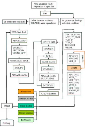
4.2.3 The Code structure... 50
4.2.4 The wetting-drying technique ... 53
4.2.5 The 2-D External Mode ... 53
4.2.6 The 3-D Internal Mode ... 53
5. Model Testing ... 54
5.1 Quarter Annular Case Test... 54
5.1.1 Quarter Annular Case Set Up on FVCOM ... 55
5.2 Physical Model... 64
5.2.1 Description of Tests ... 70
5.2.2 Physical Model Test Results... 72
5.2.3 FVCOM Validation Based on Physical Model Tests ... 77
5.2.3.1 General... 77
5.2.3.1 Lock-exchange test ... 80
5.2.3.2 25% Constriction ... 83
5.2.3.3 50% Constriction ... 84
5.2.3.4 86% Constriction ... 85
5.2.3.5 Implications to FVCOM Model... 92
5.3 Benchmark Model Grid Generation (Idealized Basin) ... 93
5.3.1 Benchmark mesh with a finite reservoir ... 98
5.4 Numerical Treatment at the Open Boundary ... 100
5.4.1 A proposed baroclinic radiative open boundary ... 102
5.5 Analysis of the pressure gradient error ... 106
5.5.1 Development of bathymetric options... 106
5.5.1.1 Flat Bottom Bathymetry ... 106
5.5.1.1.1 Water surface elevation throughout the system ... 108
5.5.1.2 Flat bottom bathymetry with a 10 m deep channel and 4 m deep open water... 109
5.5.1.3 Laterally/longitudinally changing bathymetry in the enclosed basin ... 110
5.5.2 Water surface elevation sensitivity for several different geometries... 112
5.5.3 Mass Balance of Salt in the system... 113
5.5.3.1 Salinity gradient forcing ... 113
5.5.3.2 Salinity gradient and tidal forcing... 115
5.5.3.3 Salinity gradient, tidal and hydrologic forcing ... 117
5.6 Sensitivity Analysis on the Idealized Basin... 119
5.6.1 Effect of Wind... 129
5.6.2 Effect of the number of sigma levels ... 133
5.6.2.2 Scenario 2: Parabolic distribution of the sigma levels... 136
5.7 Tidal Pumping Effect... 138
5.8 Description of the Salinity Model for the Pontchartrain Estuary. ... 142
5.8.1 Computational Grid Domain... 143
5.8.2 Model Inputs ... 144
5.8.2.1 Initial Conditions ... 144
5.8.2.2 Boundary Conditions ... 146
5.8.3 Model Calibration ... 147
5.8.4. Spatially Varying Friction... 149
5.8.4 Case Scenario: Bonnet Carré Spillway... 161
5.8.4.1 Boundary Conditions ... 161
6. Model Application ... 170
6.1 Pontchartrain Estuary, Mississippi and Alabama ... 170
6.1.2 Computational Grid Domain... 170
5.8.2 Model Inputs ... 171
5.8.2.1 Initial Conditions ... 171
5.8.2.2 Boundary Conditions ... 174
7. DISCUSSION... 182
7.1 Physical Model... 182
7.2 Idealized Basin (Benchmark test) ... 183
7.3 Radiative Baroclinic Open Boundary ... 185
7.4 Sigma pressure gradient... 187
7.5 Tidal Pumping Effect... 190
7.6 Spatially varying friction ... 191
7.7 Wind effect... 192
7.8 Salinity Transport... 196
8. CONCLUSIONS... 201
9. RECOMMENDATIONS... 204
10. REFERENCES ... 205
APPENDIX A... 211
APPENDIX B ... 638
APPENDIX C ... 666
LIST OF FIGURES
Figure 1.1 Southeastern USA. ... 1
Figure 1.2 Location of the Lake Pontchartrain Estuary... 2
Figure 2.1 Lock exchange theoretical conception ... 22
Figure 2.2 Velocity distribution in a laminar boundary layer... 25
Figure 2.3: Average shear-stress coefficients ... 26
Figure 2.4: Density contours for the (a) hydrostatic simulation and (b) non-hydrostatic simulation of the lock exchange test with Kelvin-Helmholtz billows present. ... 28
Figure 2.5 Top view and cross-section area of the linearly varying quarter annular case 32 Figure 4.1: Illustration of the FVCOM unstructured triangular grid ... 47
Figure 4.2 FVCOM flow chart... 51
Figure 4.3 Model structure of FVCOM and available modules/sub-models... 52
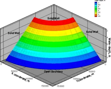
Figure 5.1 Linear bathymetry for the quarter annular case test. ... 55
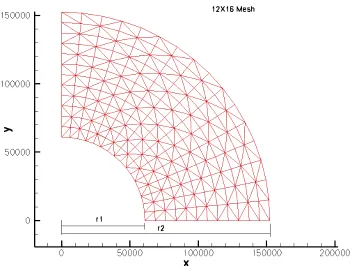
Figure 5.2 Mesh of 12x16, units in meters ... 56
Figure 5.3 Mesh of 24x32, units in meters ... 57
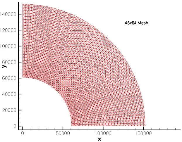
Figure 5.4 Mesh of 48x64, units in meters ... 57
Figure 5.5 Mesh of 96x128, units in meters ... 58
Figure 5.6 Treatment at corners of the domain... 59
Figure 5.7 Radial elevation profiles at =/4, t=9 days, linear bathymetry, invariant BC where is the angle measured in polar coordinates with respect to the positive r-axis ... 61
Figure 5.8 Radial velocity profiles at =/4, t=9 days, linear bathymetry, invariant BC where is the angle measured in polar coordinates with respect to the positive r-axis ... 62
Figure 5.9 Detail of the velocity profiles at the far-left end, near the Open Boundary, for =/4, t=9 days, linear bathymetry, invariant BC, where is the angle measured in polar coordinates with respect to the positive r-axis... 63
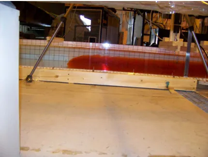
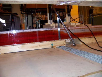
Figure 5.10: Placement of the physical model in the Hydraulics Lab... 66
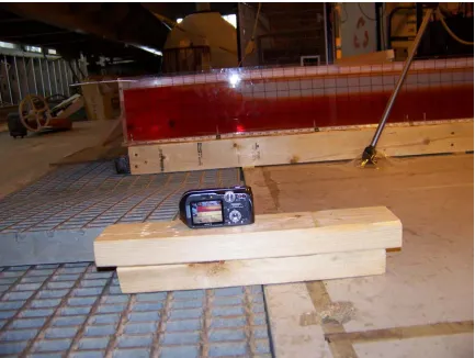
Figure 5.11: Construction of the physical model in progress ... 67
Figure 5.12: Model Setup for Lock Exchange Test Showing the Locations of the Two Sontec Doppler Current Meters ... 68
Figure 5.13: Model Setup for Lock Exchange Test Showing the Locations of the Two Sontec Doppler Current Meters ... 69
Figure 5.14: Sketch of the proposed physical model (Saline water in red). ... 70
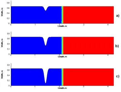
Figure 5.15: Diagram of the location of the gate and constriction for the three constricted cases: a) 25%, b) 50%, and c) 86%. [Plan view] ... 71
Figure 5.16 Constant Velocity Phase of Density Current... 72
Figure 5.17 Downstream Rebound of Density Current ... 73
Figure 5.18 Traveling Internal Hydraulic Jump of Density Current ... 74
Figure 5.19 Internal Wave in Nearly Stratified Flow ... 75
Figure 5.20: Observed speeds of propagation for fresh and saltwater plumes in the lock exchange test... 76
Figure 5.21: Distribution of the sigma levels using a parabolic function... 79
seconds... 79
Figure 5.23: Speed of propagation versus time of the lock-exchange test with 21 sigma levels ... 81
Figure 5.24: Advancement of the saltwater plume in the lock exchange test for both the experiment and numerical cases [side view]. Note: the FVCOM Images have greater vertical distortion. ... 82
Figure 5.25: Speed of propagation versus time of 25% constriction case with 21 sigma levels ... 84
Figure 5.26: Speed of propagation versus time of the 50% constriction case with 21 sigma levels... 85
Figure 5.27: Speed of propagation versus time of the 86% constriction case with 21 sigma levels for Scenario 4. ... 87
Figure 5.28: Advancement of the saltwater plume through the 86% constriction for both the experiment and FVCOM (Plan view). Note: longitudinal scale is compressed relative to the Physical Model... 88
Figure 5.29: Profile showing salinity interface for Scenario 4. ... 89
Figure 5.30: Kelvin-Helmholtz instabilities developed in the case with a constricted width of 86% [Side view] ... 91
Figure 5.31: Holmboe instabilities developed in the lock exchange test case [Side view] ... 91
Figure 5.32: Degrees of stratification after reaching equilibrium... 93
Figure 5.33: The Lake Pontchartrain System ... 94
Figure 5.34: Bathymetry of Chef Menteur Pass. ... 95
Figure 5.35: Bathymetry of Pass Manchac... 96
Figure 5.36: Bathymetry of The Rigolets Pass. ... 96
Figure 5.37: Salinity contours at the initial condition and 3-D mesh for the idealized case showing the unstructured grid with a parabolic distribution of the sigma levels ... 99
Figure 5.38 shows transcritical internal flow at the constriction followed a hydraulic jump that was generated when the saltwater plume flows through the tidal pass... 100
Figure 5.39: Failure of the code when the freshwater plume reaches the open boundary. ... 102
Figure 5.40: Computational time-space grid for outflow/inflow conditions ... 104
Figure 5.41: Coarse resolution benchmark grid with a flat bottom and an average depth of 4.0m ... 106
Figure 5.42: Water surface elevation for location (0, 0) at the center of the enclosed basin. Hourly output... 108
Figure 5.43: Water elevation for the Pontchartrain System for a diurnal tide. Hourly output. ... 109
Figure 5.44: Idealized basin with flat bottom of 4m and an interconnecting channel 10m deep... 110
Figure 5.45: Radially changing bathymetry in the enclosed basin ... 111
Figure 5.46: Water surface calibration performed for the three bathymetries. Hourly output. ... 113
Figure 5.47: Mass Balance of salt with only density gradient forcing. Daily output. .... 115
Figure 5.49: Mass Balance of salt with density gradient, tidal and hydrologic forcing. Daily output. ... 119 Figure 5.50: Comparison of water surface elevations at the enclosed basin for variable external time steps. Hourly output... 121 Figure 5.51: Comparison of water surface elevations at the enclosed basin for variable ISPLIT (ratio of internal to external time step). Hourly output... 122 Figure 5.52: Comparison of water surface elevations at the enclosed basin for a 3-D grid structure and a 2-D grid structure. Hourly output... 123 Figure 5.53: Comparison of water surface elevations at the enclosed basin for variable bottom shear stress coefficient. Hourly output. ... 124 Figure 5.54: Comparison of total mass of salt in the system for variable bottom shear stress coefficient. Hourly output... 125 Figure 5.55: Comparison of total mass of salt in the system for variable horizontal
diffusion i.e., Smagorinsky eddy parameter HORCON. Hourly output... 126 Figure 5.56: Comparison of total mass of salt in the system for constant, and Mellor-Yamada level 2.5 diffusivities in the vertical turbulence model. Daily output. ... 127 Figure 5.57: Comparison of total mass of salt in the system for variable vertical eddy viscosity “UMOL”. Hourly output. ... 128 Figure 5.58: Comparison of total mass of salt in the system for the variation in the
advection scheme. ... 129 Figure 5.59: Comparison of total mass of salt in the system for a) Flat bottom bathymetry with wind b) Laterally/longitudinally changing bathymetry in enclosed basin with wind. ... 130 Figure 5.60: Flow field at 2.2m deep for the geometry with laterally/longitudinally
changing bathymetry in the enclosed basin. Wind is 7 m/s 121º north-based azimuth at the 543rd hour of simulation time... 132 Figure 5.61: Flow field at 2.2m deep for the geometry with laterally/longitudinally
Figure 5.71: Tributary flows used in the model. Flows represent a 17 year average of the
mean daily flow for each day... 147
Figure 5.72: Monitoring stations in the system utilized to collect water surface elevation and salinity values... 148
Figure 5.73: Tidal discharge surveys through the passes, August 1997. Flows are in cfs x 1000... 149
Figure 5.75: Salinity calibration in Lake Pontchartrain at LUMCON (2003). Daily output. ... 155
Figure 5.76: Mass of Salt in the Pontchartrain System for a year. Daily output. ... 156
Figure 5.77: Simulated surface salinity for the freshest condition in the system during the year (March 15th) ... 158
Figure 5.78: Simulated surface salinity for the most saline condition in the system during the year (December 11th)... 159
Figure 5.79: Surface salinity at the 365th Julian day of the simulation time... 160
Figure 5.80: Bottom salinity at the 365th Julian day of the simulation time... 161
Figure 5.81: Bonnet Carré Spillway discharge for the 2008 opening. (J. Lopez, 2008) 162 Figure 5.82: Forced tide at the Open Boundary... 163
Figure 5.83: Wind speed at the LUMCON station located northwest of the Lake Pontchartrain ... 164
Figure 5.84: Direction from where the wind is blowing with respect to the north-based azimuth... 165
Figure 5.85: Comparison of the water surface elevation for April and May 2008 at the LUMCON monitoring station in Lake Pontchartrain. Hourly output... 166
Figure 5.86: Percentage of change due to the opening of the Bonnet Carré Spillway between the observed and modeled salinity values. ... 167
Figure 5.87: Surface salinity pattern in the Pontchartrain Basin on April 29th, 2008... 168
Figure 5.88: Satellite image on April 29th, 2008 showing the sediment propagation due to the 2008 opening of the Bonnet Carré Spillway... 169
Figure 6.1: Model computational domain composed by 22882 cells and 12281 nodes . 171 Figure 6.2: Model Bathymetry relative to MSL ... 172
Figure 6.3: Initial condition for surface salinity used in the model. ... 173
Figure 6.4 Tributary flows used in the model... 175
Figure 6.5: Annual variation in salinity (FVCOM) at selected stations ... 177
Figure 6.6: Surface Salinity Distribution at minimum system salinity... 178
Figure 6.7: Surface Salinity Distribution at maximum system salinity... 179
Figure 6.8: Surface Salinity Distribution at the end of one year. ... 180
Figure 6.9: Bottom Salinity Distribution at the end of one year... 181
Figure 7.1 Velocity vector field at the open boundary [side view]. Salinity in ppt... 186
Figure 7.2: Mass Balance of salt with density gradient, tidal and hydrologic forcing. Hourly output. (from Figure 5.49) ... 189
Figure 7.3: Comparison of total mass of salt in the system for various constant wind speeds... 193
Figure 7.4: Upwelling and downwelling due to 1 m/s southerly wind in the enclosed basin for an isosurface of 2 ppt. ... 194
Figure 7.6: Comparison of total mass of salt in the system with fine resolution for
LIST OF TABLES
Table 2.1: Analytical forms of the barotropic OBC ... 18
Table 2.2: Comparison between the Froude numbers of the non-hydrostatic and hydrostatic simulations ... 29
Table 5.1 Real time for a total simulation time of 9 days for the different meshes with a time step of 4s (3 sigma levels)... 61
Table 5.2 Constriction profiles for the projected runs ... 71
Table 5.3 Speed of propagation for the saltwater density current ... 76
Table 5.4: Speeds of the saltwater density current for the observed data... 77
Table 5.5 Grid Resolution and Initial Conditions for the FVCOM and Physical Tests ... 78
Table 5.6: Root Mean Square speed of propagation for the primary saltwater density current ... 81
Table 5.6: Root Mean Square velocities for the saltwater density current for the observed data... 83
Table 5.7: Hydraulic characteristics of the main lakes in the Pontchartrain Estuary ... 97
Table 5.8: Hydraulic characteristics of the main channels in the Pontchartrain Estuary . 97 Table 5.9: Hydraulic parameters for the equivalent lakes and channel to be used in the benchmark grid for a flat bottom bathymetry 4-m deep. ... 107
Table 5.10: Times at which the simulation will reach a background salinity of 25ppt in the system... 116
Table 5.11: Water surface elevation and Flow calibration for various shear stress coefficients in several different areas. ... 151
Table 5.12: Observed and simulated flows for the main passes between Lake Borgne and Lake Pontchartrain... 151
Table 5.13 Observed and simulated tidal ranges and phases for the spring tide. ... 152
Table 5.14: Observed and simulated average salinities over a one year period ... 153
Table 5.15: RMS and RMSE values of simulated and measured water surface elevation at the LUMCON station in Lake Pontchartrain... 166
Table 6.1 Observed and simulated tidal ranges for the spring tide... 176
NOMENCLATURE
Symbol Description Units
Density M/L3
Velocity Z-direction L/T
Kinematic viscosity L2/T
Bottom shear stress M/L/T2
Water surface elevation L
Divergence operator L-1
Angular frequency T-1
Angular polar coordinate T-1
Standard deviation
Conserved quantity
k Turbulent Prandtl number Dimensionless
TCE; MCE Tracer and Momentum control elements,
respectively
L2
A Area L2
Ah Horizontal thermal diffusive term L2/T
Am Horizontal eddy coefficient L2/T
ao Tidal amplitude L
c Surface phase speed L/T
c1,c2.c3 Coefficients in the k-ε turbulent model
cbc Baroclinic phase speed L/T
Cf Bottom shear stress coefficient Dimensionless
D Total water column L
E1; W Coefficients in the “q-ql” turbulent kinetic model
F Froude number Dimensionless
f Coriolis parameter T-1
F` Densimetric Froude number Dimensionless
Fl Horizontal diffusion of the macroscale L3/T3
Fq Horizontal diffusion of the turbulent kinetic
energy
L2/T3
FS Salt diffusion term M/L3/T
FT Thermal diffusion term M/L3/T
Fu Horizontal momentum in the X-coordiante L/T2
Fv Horizontal momentum in the Y-coordiante L/T2
Fx Horizontal diffusion term in the X-coordinate M/L3/T
Fy Horizontal diffusion term in the Y-coordinate M/L3/T
g Gravity L/T2
G Turbulent buoyancy production in the k-ε
turbulent model L
2/T3
g` Reduced gravity L/T2
H n (1) Hankel function of the first kind for the “n” order
H; h Water depth L
hc Water depth of tidal pass L
Hn(2) Hankel function of the second kind for the “n”
order
i Imaginary unit
J1 Bessel function of the first kind for the first order
J2 Bessel function of the first kind for the second
order
Kh Thermal vertical eddy diffusion coefficient L2/T
Km Vertical eddy viscosity coefficient L2/T
Kq Vertical eddy diffusivity of the turbulent kinetic
energy
L2/T
L Length of the plate L
l Turbulent macroscale L
P Pressure M/L/T2
P Turbulent shear production in the k-ε turbulent
model L
2/T3
Pb Buoyancy production term of the turbulent kinetic
energy
L2/T3
Ps Shear production term of the turbulent kinetic
energy L
2/T3
q2 Turbulent kinetic energy L2/T2
r Radial polar coordinate L
Rex; ReL; Re Reynolds number Dimensionless
S Salinity M/L3; M/M [ppt]
t Time T
Tf Friction time scale T
U, u Velocity X-direction L/T
v Velocity Y-direction L/T
vn Normal velocity L/T
Vr Radial velocity L/T
vt Turbulent viscosity L2/T
x X Cartesian coordinate L
y Y Cartesian coordinate L
Y1 Bessel function of the second kind for the first
order
Y2 Bessel function of the second kind for the second
order
z Z Cartesian coordinate L
zab Half thickness of the bottom sigma layer Dimensionless
zo Bottom roughness L
ε Turbulent kinetic energy dissipation rate L2/T3
ABSTRACT
The objective of this study was to develop a 3-D model for The Pontchartrain
Estuary that was capable of long-term mass conservative simulation of salinities. This
was accomplished in a multi-stage approach involving: a physical model of salinity
exchange through a pass; a 3-D FVCOM model of the physical experiment; the
development and testing of an FVCOM model for an idealized Pontchartrain Basin; and
for the entire estuary.
The data from the physical model tests were used to validate the performance of
the FVCOM model with density-driven flows. These results showed that hydrostatic
FVCOM captured the primary internal wave movement. The idealized basin simulations
were used to evaluate several issues related to salinity transport, namely the relative
importance of baroclinic forcing, tidal forcing and hydrology. The idealized domain also
permitted the testing of sigma-gradients, spatial distribution of friction coefficients, wind
stress and various boundary treatments. The results showed that the density-driven
exchange of saltwater at the open boundary required a baroclinic boundary condition for
salinity as well as a lateral filter at the boundary on each sigma layer. A new radiative
baroclinic open boundary condition was developed for FVCOM.
When tides and hydrology were included, the FVCOM model was shown to
reproduce the seasonal salinity that has been observed for long-term periods. It was also
water regions and high friction was needed in the passes and waterways to reproduce the
tides and salinity distribution. A variable friction coefficient option was coded on
FVCOM.
The findings from the idealized model were utilized to setup two models for the
actual estuary. Both models extend from Lake Maurepas, one to the Chandeleurs Islands
and the other to Mobile Bay. The baroclinic open boundary and variable friction were
implemented in these models. They were calibrated for tides and salinity. The 2008
Bonnet Carré Spillway Opening was applied to the first model. A tidal pumping effect in
Lake Pontchartrain was observed and captured by the model.
Keywords: Pontchartrain Estuary, Salinity Model, Baroclinic Open Boundary,
1. INTRODUCTION
1.1 Background
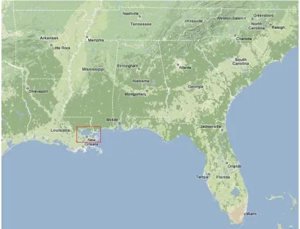
The Pontchartrain Estuary is a brackish estuarine located in Southeastern
Louisiana, USA. It is comprised by three major lakes: Lake Pontchartrain, located to the
north of New Orleans; Lake Maurepas, connected to its west end through Pass Manchac;
and Lake Borgne, connected to its east end through two major tidal passes, the Rigolets
and Chef Menteur. Figures 1.1 and 1.2 show the location of the estuary.
Figure 1.2 Location of the Lake Pontchartrain Estuary. Source: Louisiana Department of Natural Resources.
Habitats for fish, shells, and clams in the estuary are sensitive to saline patterns.
In fact, increased lake salinities due to saltwater intrusion have significant impacts on the
lakes ecosystem. The salinity distribution in Lake Pontchartrain is governed by
freshwater inputs from rivers, canals, rainfall, Mississippi diversions, and thermal
evaporation (Georgiou, 2002).
Several different hydrodynamic and numerical transport models, such as
RMA10-WES (McAnally et al., 1996), POM (Georgiou, 2002), RMA2/RMA4 (Haralampides,
estuary. However, little attention has been given to the radiation of salinity at the Open
Boundary (OB). In fact, modelers have assumed that not only the open boundary would
properly radiate out the conserved quantity , such as salinity, but also the conserved
quantity would be preserved locally and globally.
There is evidence that the “pressure gradient error” of sigma-coordinates in
association with fully unstructured grids (Fringer et al., 2006) can lead to significant
errors in the model results. Haney (1991) noted that the pressure gradient force is the sum
of two terms. One term involving the gradient of pressure along a constant sigma-surface
and one that involves the gradient of bathymetry. If the topography is steep these terms
become large with opposite signs. Thus, the mathematical representation of the terms
leads to a small error in computing any of these terms, and consequently, results in a
large error in the total pressure gradient force (Haney, 1991; Mellor et al., 1994). In
addition, the approximation of the horizontal diffusion terms in the governing equations
can generate to additional vertical mixing in the sloped regions for the sigma coordinate
(Chen et al., 2006). Moreover, model results are directly influenced by the imposition of
the forcing at the open boundary. Chapman (1985) summarizes several different
treatments of the radiative open boundaries for barotropic models. Radiative open
boundaries should allow the motion of the fluid to be unrestricted, such that perturbations
in the conservative quantity , generated within the domain, should be able to propagate
outside of the domain when they reach the open boundary without generating artificial
reflections into the model domain. However, these studies have mainly been focused in
gravity waves, e.g., due to salinity.
1.2 Problem Statement
The salinity distribution and hydrodynamics of the Pontchartrain Estuary have
been simulated using several different 2-D and 3-D computational fluid dynamic models
with different discretization methods (e.g., difference, element,
finite-volume). These developments have used structured and unstructured grids; however, the
use of unstructured grids in combination with finite-volume method schemes has gained
popularity due to the possibility of not only discretizing more complex geometries, but
also because the finite-volume method mathematically ensures conservation of
transportable variables by solving the governing equations in their integral form using
flux computations.
New developments in computing technologies have introduced the concept of
applying multiple processors for the execution of Computational Fluid Dynamic (CFD)
models. This technique is called parallelization and leads to the speeding up of the
solution by decomposing the domain geometry in subdomains where each subdomain is
assigned a processor.
The Finite-Volume Coastal Oceanographic Model (FVCOM), a 3-D
sigma-coordinate based model, has been selected to simulate hydrodynamic and salinity patterns
of the Pontchartrain Estuary. Unstructured domain of the code can be better suited to the
tidal passes, inlets, and irregular coastline of Southeast Louisiana. In addition, the code
mentioned, there is evidence that sigma-coordinate based models are associated with the
“pressure gradient error” when the bathymetry of the system is steep. Besides, the
approximation of the horizontal diffusion terms in the primitive equations can generate
additional vertical mixing in steep bathymetry with sigma-coordinates.
In addition, although there is literature regarding propagation of the water
elevation and velocity out of the computational domain (Chapman, 1985), less attention
has been given to radiative open boundaries for internal gravity waves e.g., due to
salinity. Consequently, salinity distributions within the computational domain may be
improperly predicted because the interior salinity depends on the correct physical
treatment of the open boundary.
Moreover, the lack of radiation of internal gravity waves in CFD models may
result in reflection of these waves. In estuaries, inputs from freshwater diversions and
river discharges are common. These freshwater density flows tend to travel in the top
vertical layers of the water column. However, lighter density flows may not be able to
travel out through the open boundary if the model does not offer an open boundary
capable of radiating internal waves. In fact, the lighter density flow would be trapped
within the system. As a result, accumulation of lighter trapped density flows would lead
1.3 Significance
The current study makes two main contributions to the scientific community.
Firstly, from the point of view of numerical modeling, this research proposes a general
baroclinic numerical treatment of the open boundary. This new baroclinic condition is
capable of radiating freshwater and saltwater density currents across the open boundary
for an unstructured grid model. Secondly, the development of a model for the
Pontchartrain Estuary that simulates long term salinity helps to predict changes in the
salinity regime induced by Mississippi River diversions, and drought periods.
In addition, a variable friction coefficient was coded to properly reproduce the
relatively low friction required in the open water regions and the higher friction needed in
tidal passes and waterways to reproduce tides and salinity through out the estuary.
The model also identifies and quantifies the significant increase of the mean water
level in the enclosed basin, due to combined effects of tidal pumping and freshwater
inputs.
1.4 Objectives
The overall project objective is to develop a model for a tidal estuary with
constrictive tidal passes that is capable of simulating long term salinity. The
Pontchartrain Estuary will be used as the physical domain for the evaluation of the
The specific objectives of the proposed study are:
To investigate, with the aid of a physical model, the propagation and radiation of
an internal gravity wave through a constriction.
To develop a radiation boundary condition for the internal gravity waves
(baroclinic OBC).
To develop a model for an idealized estuary consisting of an enclosed basin,
semi-enclosed basin and narrow passes for benchmark testing. Testing includes:
1. the sensitivity to the bathymetric pressure gradient error.
2. the system response in a presence of the constrictive tidal pass.
3. the system response to the proposed radiative open boundary.
To evaluate the mass conservation of salinity for changes in sigma gradients. The
system will have the new OB treatment implemented.
To develop a three-dimensional model with a radiative open boundary condition
for internal gravity waves capable of simulating salinity in the Pontchartrain
Estuary.
To prove the applicability of the revise model by application to the entire
1.5 General Methodology and Research Plan
The following methodology was used to meet the proposed objectives:
1. A literature review was conducted.
2. Selection criteria were applied to choose the best numerical model.
3. An idealized estuary was designed for benchmarking purposes
4. A physical model was constructed to measure the speeds of propagation of
the exchange flows in a system with a constriction.
5. The effect of the pressure gradient, boundary conditions, and a tidal pass
were evaluated using an idealized estuary and an unstructured grid. The
idealized basin will be hydraulically similar to the Pontchartrain Estuary.
6. The selected three-dimensional, sigma-layer, unstructured grid, numerical
model capable of simulating hydrodynamics and the dynamics of salinity
fate and transport was set up for the physical model, the benchmark mesh,
and the Pontchartrain Estuary.
7. The development of a numerical treatment for the radiation of
density-driven flows at the open boundary was implemented in the model and
tested with the idealized estuary.
8. A spatially varying shear stress coefficient for friction was implemented in
the model.
9. Calibration and verification of long-term simulations for the Pontchartrain
Estuary were performed to evaluate the conservative characteristics of the
code with regard to the distribution of salinity.
Mississippi Sounds. Its results were validated based on the available data
from LUMCON, NOAA, USGS and US Army Corps of Engineers
2. LITERATURE REVIEW
2.1 General
The use of the Finite Volume Method (FVM), in the Computational Fluid
Dynamics Field (CFD), has gained popularity in recent years because the control volume
integration guarantees conservative properties. In addition, FVM in combination with the
use of unstructured grids offers the possibility of easily discretizing very complex
geometric configurations compared to the structured grids (Kobayashi et al., 1998).
Essentially, CFD codes are structured around the numerical algorithms that can
solve fluid flow problems. Typically, CFD codes contain three main elements: a
pre-processor, a solver, and a post-processor (Versteeg and Malalasekera, 1995).
Pre-processing procedures are:
1. the definition of the geometry of the area of the study commonly known as
computational domain,
2. the subdivision of the domain into smaller non-overlapping cells or grid (or
mesh) generation,
3. the selection of the transportable quantities (state variables) related to the
transport phenomena,
4. the initial state of the fluid properties, and
The solver, using a numerical algorithm, integrates the governing equations of
fluid flow over the control volumes or cells. This algorithm leads to a system of algebraic
equations which are formulated in discrete space by finite-difference, finite-volume or
finite-element type approximations. The system of algebraic equations is often solved by
iterative methods, providing information about the flow state.
Finally, post-processing involves the visualization tools that process the output of
the solver.
2.2 Conservativeness
Conservation statements express the fact that certain physical quantities of a given
system must be preserved during any given physical process. Conservation statements
normally take into account the time rate of change of the conserved quantity . The time
rate of change of a quantity is related to the physical process occurring within the system
and/or at the system boundaries.
Versteeg and Malalasekera (1995) indicate that successful CFD simulations are
obtained by ensuring schemes that posses the conservativeness, boundedness and
transportiveness properties. Perhaps, the most notable characteristic of the finite volume
method is its conservativeness. The finite volume approach ensures local conservation of
throughout the entire domain.
Integration of the governing equations over the control volumes gives a set of
discretized conservative equations involving fluxes of the conserved quantity through
the faces of the control volume. To ensure conservation of for the whole solution
domain the net transport of the conserved quantity out of the control volume is equal to
the flux of the conserved quantity across the control surface (the flux of a quantity is the
amount of a quantity that crosses a unit surface area per unit time). Moreover, the flux of
leaving a control volume through the face must be equal to the flux of entering the
adjacent control volume through the same face. In fact, the evaluation of the flux
components on the sides of the cells depends on the selected interpolation scheme as well
as on the location of the flow variable in the grid. The most common schemes used in
Finite Volume Methods are the central and the upwind discretization schemes. The
central scheme is based on local flux estimations, whereas the upwind scheme computes
the fluxes according to the direction of the propagation (Hirsch, 1988).
The governing equations are statements of conservation laws, and since these
equations can be solved in their integral form by flux calculations, they ensure
conservation of the transported quantity in both the individual control volume and the
overall computational domain. The conserved quantity is preserved or, at least, varies
2.3 Sigma-Coordinate and Pressure Gradient
Sigma-coordinates, also known as terrain-following coordinates, were developed
approximately 20 years ago to satisfy the need of simulation of flows in estuaries and
coastal regions with the incorporation of turbulent processes (Ezer et al., 2002). The
coordinate system has attracted the attention of ocean modelers because of its smooth
representation of topography and its ability to simulate interactions between flows and
topography (Mellor et al., 2002). In contrast, Ezer, et al., (2002) indicate that z-level
models have shown a step-like representation of the bathymetry and some difficulties
simulating flow over an irregular surface.
For instance, in simulating the downslope spreading of a dense plume on a bottom
boundary layer, Ezer and Mellor (2004) state that the dynamics are “dominated by the
along-sigma advection driven by pressure gradients, with a thin and stably stratified
bottom boundary layer” for sigma-coordinates. In z-level coordinates the process is
dictated by “a combination of horizontal advection and diffusion that creates
hydrostatically unstable columns over the stepped topography that results in intense
vertical mixing and thicker boundary layers”. This could be overcome by an appropriate
VOF, e.g. as in Flow3D.
Nevertheless, Haney (1990) points that a pressure gradient error is observed with
sigma coordinates when the bathymetry is steep. Haney suggests that the pressure
gradient force is the sum of two terms. One term involves the gradient of pressure along a
the slope of the bathymetry becomes large, these terms also become large, but with
opposite signs. Therefore, a small error in computing either term in these conditions
results in a large error in the total pressure gradient force.
Mellor et al., (1994) suggest that the horizontal pressure gradient variation is
influenced by both the vertical and horizontal resolution. In fact, Mellor et al., (1994 and
1998) propose that the sigma-coordinate, pressure gradient error decreases with the
square of the vertical and horizontal grid size. In addition, they have shown that the initial
pressure gradient error is advectively eliminated after a long integration; however,
density errors are created, which affect the salinity and temperature fields. On the
contrary, Weisberg and Zhen (2006) state that by flux analysis of water and salt through
various cross-sections of Tampa Bay, FVCOM ensures conservation of mass over long
simulations intervals.
2.4 Boundary Conditions
Treatment of the boundary conditions addresses how many conditions of a
physical nature origin are to be imposed. Actually, these conditions should be determined
by the physical set up. Specification of too few or too many conditions, or inappropriate
conditions would make the mathematical problem an ill-posed problem. As a result, an
ill-posed problem would have either no solution, or many solutions for the same set up
(Leveque, 2002). In addition, boundary conditions are to be formulated and discretized to
be compatible with the order of accuracy and stability conditions of the interior
According to the Hadamard principle, to have a well-posed problem to a system
of equations, the necessary information must be imposed on the initial and boundary
conditions such that the solution depends, in a continuous way, on the initial and
boundary conditions i.e., a small perturbation of these conditions should prompt to a
small variation of the solution at any point of the domain at a distance from the
boundaries (Hirsch, 1988).
The physics of a CFD problem should dictate the nature of the boundary
conditions that should be specified. The most common boundary conditions are as
follows:
wall
inlet (inflow)
outlet (outflow)
prescribed pressure
2.4.1 Wall or Solid Boundary Conditions
According to Veersteeg and Malalasekera (1995), this is the most common
boundary found in a confined system. Normal fluxes and flow variables are usually set to
zero. Tangential velocities may be treated by full slip (no shear), partial slip or no slip
(full shear). When shear stresses play a significant role, boundary layer theory must be
2.4.2 Inlet Boundary Conditions
Typically, the inlet boundary is specified in one of the edges of a domain. The
distributions of the flow variables should be externally specified. Thus the information
required to perform the computation should travel into the system.
2.4.3 Outflow Boundary Conditions
At these boundaries, no external signal should be applied. The information at this
boundary comes from what is being computed inside of the domain. Furthermore,
outgoing waves that arrive at this boundary should leave the domain cleanly without
creating spurious reflections back into the system (Leveque, 2002). It is noted that an
outflow boundary may become an inflow boundary under some circumstances; this case
is treated under ‘Open Boundaries’.
2.4.4 Constant or Specified Pressure Boundary Conditions
Free surface flows and density-flows are applications where a constant pressure
boundary condition is used. Typically, when the details of the flow distribution are
unknown but the pressure of the boundary values is known (Versteeg and Malalasekera,
2.5 Open Boundaries
In coastal ocean problems, typically inlet or outlet boundary conditions are
imposed. These types of boundary conditions are also called Open Boundaries Conditions
(OBC). Chapman (1985) considered different types of barotropic OBC to radiate out of
the computational domain water surface elevation and velocity.
2.5.1 Barotropic OBC
The analytical expression for a barotropic OBC is a Sommerfeld type radiation
condition described as:
x c t or c x
t
(2.1)
where is the conserved variable, and c is the phase speed . For this case, water surface
elevation and velocity. Table 2.1 shows the analytical forms of the possible barotropic
Table 2.1: Analytical forms of the barotropic OBC (After Chapman, 1985)
Open Boundary Condition Analytical form Phase speed (c)
Clamped (CLP) 0 n/a
Gradient (GRD) x 0 n/a
Gravity-wave
radiation(GW(1)): t cx 0 c gh
Partially clamped(BK(1),(2)):
f x
t
T
c
c gh
Orlanski radiation(OR(1),(3)):
0
x
t c
0 0 0 x t x t x t x t if t x if t x if t x c
(1) Explicit or Implicit
(2)Blumberg and Kantha (1982) (3) Orlanski (1976)
x=the grid spacing; t=the time step; g=gravity; h=water depth; Tf=a friction time scale to slow down the emptying of the basin.
According to Chapman (1985), the CLP and GRD conditions are perfect
reflectors in which the amplitude of the reflected waves is equal to the amplitude of the
incident wave. If a reflected wave is generated, it remains inside of the computational
domain until either bottom friction damps it out or it encounters another open boundary
where part of the wave may be radiated through the boundary and part may be reflected
back into the system (Chapman, 1985). On the other hand, the ORI and ORE conditions
2.5.2 Baroclinic OBC
Little literature regarding baroclinic OBC is available. However, Rochford and
Shulman (2000) suggested a numerical treatment for the baroclinic velocities and salinity
implemented in the Pacific West Coast, version of the Princeton Ocean Model as
developed at the Naval Research Laboratory. Their analytical form of the radiative
baroclinic velocities or salinities is as follows:
gh c
where
cbc n bc
t 1000 5 0
(2.2)
where is the salinity or the normal velocity to the OB; n is the coordinate in the
direction normal to the OB; cbc is the baroclinic phase speed, as a fraction of the
barotropic phase speed .
If is salinity S, the normal gradient of the salinity is given by:
) ( ) (inf 0 0 outflow v n S S low v n S S n S n i n (2.3)
n is the grid spacing normal to the OB, vn is the normal velocity; Si the salinity at one
grid point inside the OB; S0 is the user specified salinity at the OB, and S is the salinity
applied along the open boundary.
Rochford and Martin (2001) also suggested a similar treatment for the Navy
For normal baroclinic velocity, four boundary conditions are provided as follows:
Internal Model Calculated Value: the model computes the normal baroclinic
velocity at the OB using the same calculation as for the internal velocity points.
Orlanski Radiation: an Orlanksi radiation condition is used to set the normal
baroclinic velocities at the OB for outward propagation, whereas a relaxation to
an already prescribed value is used for inward forcing.
Internal Model Calculated plus Advection: the model calculation of the normal
baroclinic velocity at OB is used when the propagation is outward. A relaxation to
a prescribed normal velocity is used when the propagation is inward.
Advective-Radiative: this is similar to the previous case but the radiative
propagation of the normal velocity is applied as in equation (2.2) with the
baroclinic phase speed cbc.
For the salinity, four boundary conditions are also provided as:
Prescribed values: the model places the externally prescribed values on the OB.
This treatment behaves as a reflective boundary.
Orlanski Radiation: for outflow propagation the Orlanski radiation condition is
applied. An externally prescribed value is applied at the OB with a relaxation
method for inward forcing.
Advective: A similar treatment to equation (2.2) is applied, but instead of using
Advective with Vertical Advection: it is applied for cases with strong upwelling
or downwelling along the open boundary. Therefore, the horizonal gradient x is
being replaced by the vertical gradient z. The phase speed is the vertical velocity.
2.6 Flow of Density Current
The propagation of any internal gravity wave is important when dealing with
systems where the transport of salinity is affected by density gradients such as in a
brackish system like the Lake Pontchartrain System. The movement of denser fluid (salt
wedge) has been observed in navigation channels near the coast such as the Mississippi
River Gulf Outlet (MRGO) (Georgiou and McCorquodale, 2000). In this case a saltwater
plume advances into the system in the bottom of the water column (underflow) and a
lighter fluid advances on the opposite way in the top layers (overflow).
The lock-exchange flow test is useful to assess the capability of the code to
properly simulate the propagation of internal gravity waves. Initially, two volumes of
water at rest with different densities (freshwater and saltwater) are separated by a gate.
After opening the gate the freshwater is displaced by the saltwater at the bottom and,
conversely, the saltwater is displaced by the freshwater at the surface. Figure 2.1 shows
Figure 2.1 Lock exchange theoretical conception
Specifically, gravity converts the potential energy into the kinetic energy that
drives the current, also known as density current. Thus, the saltwater sinks and the fresh
water is raised (van Rijn, 1990). By equating the decrease in potential energy with the
increase in kinetic energy and neglecting friction effect, the theoretical speed of
propagation Uo can be calculated such that:
gH Uo
0.5 (2.4)
and the densimetric Froude number defined by Shin et al., (2004) can be determined as:
1 h g U
F o
where 2 1 2 g
g (2.6)
H is the total water depth; h1 is the thickness of layer 1; 1 is the density of layer 1; 2 is
the density of layer 2 (largest density); g is the gravity; and g΄ is the reduced gravity.
Furthermore, Simpson (1987) has shown that density currents produced by
instantaneous release undergoes two different phases, a constant speed phase and
self-similar flow phase. The constant speed phase is produced after the gate is removed. In
this phase, the front advances at constant speed, and the fluid left behind forms an
internal gravity wave. The mixed fluid left behind is confined to a region just behind the
leading edge of the front. In addition, there is an acceleration phase that precedes the
constant velocity phase.
According to van Rijn (1990), Armi (1986), and Schijf and Schönfeld (1953), the
speed of propagation “c” of the internal gravity waves along the interface of the layers of
different densities is described by:
22 1 2 1 2 1 2 2 1 2 1 1 1 2 2 1 1 2 2 1 h h h h u u h h h h g h h h u h u c (2.7)
where ū1 = depth-averaged velocity of layer 1; ū2 = depth-averaged velocity of layer 2
(denser layer); h1 = thickness of layer 1; and h2 = thickness of layer 2 (denser layer).
Typical propagation velocities of internal gravity waves in full-scale systems are
waves can become large. Therefore, the currents generated by internal gravity waves can
also be large and sometimes exceeding the tidal current velocities. Milne-Thomson
(1968) indicates that when the densities are nearly equal, the periods of oscillations of the
common surface are also long, compared with the period of oscillations of surface waves
in which the density difference between air and water is quite large.
2.6.1 Energy Dissipation in Density currents
The movement of a denser fluid under a light fluid generates energy dissipation at
the interface of the two exchanging flows. Wilkinson and Wood (1972) state that the
propagation of the leading edge is determined by the interfacial and boundary frictional
forces acting on the layer behind the head. They found that density interfaces can modify
the shape and rate of advancement of density currents. Moreover, during the initial
motion the flow is largely unaffected by viscous forces that will play a major role once
that the gravity current has travelled some distance.
Benjamin (1968), Wilkinson and Wood (1972) showed that the only energy conserving
case is when h1=h2, and neither dissipation, nor wake zone are observed. Flows of
density currents in which h1 is less than h2 are not physically realistic and energy of
density currents in which h1 is greater than h2 is lost in the wake immediately behind the
leading edge. Furthermore, they suggest that energy may be dissipated in the form of
interfacial waves, and the dissipation and degree of turbulence are related to the
2.6.2 Bottom Boundary layer resistance
The resistance created by the bottom solid surface affects the boundary layer. A
boundary layer is described as the region next to the surface of an object in which the
velocity of the fluid decreases due to the shearing resistance i.e., shearing stress
(Roberson and Crowe, 1990). Blasius (1908) obtained a solution for flow in a laminar
boundary layer, in which the viscous effects are concentrated in the layer next to the solid
boundary. He proposed an invariant shape of a non-dimensional velocity distribution
across the plate. Figure 2.2 shows the non-dimensional velocity distribution in a laminar
boundary layer, where x is distance from the leading edge of the surface, Uo is the free
stream velocity, u is the velocity near the boundary layer, is the kinematic viscosity, y is
the vertical distance from the bottom, and Rex is the Reynolds number defined as follows:
x Uo
x
Re (2.8)
The shear stress at the boundary, o, can be express in terms of a dimensionless
coefficient Cf, and the dynamic pressure of the free stream. The shear stress and the
dimensionless friction coefficient are expressed in equation 2.9, and 2.10, respectively.
2
2
0 f o
U
c
(2.9)
x f
c
Re 33 . 1
(2.10)
Figure 2.3 shows a plot of the friction coefficients for the laminar, turbulent, and a
combination of laminar and turbulent boundary layers developed by Schlichting (1979). L
represents the length of the plate. Roberson and Crowe (1990) suggest that the transition
or critical region on a smooth plate occurs at a Reynolds number of approximately
500,000.
2.6.3 Kelvin-Helmholtz and Holmboe instabilities
In a symmetric, stably stratified, free shear layer i.e., “one in which the shear and
the stratification are distributed symmetrically about some central level” (Smyth and
Peltier, 1989), energy dissipation may occur due to Kelvin-Helmholtz or Holmboe
instabilities which depend on the conditions of the background stratification (Smyth and
Peltier, 1989). For instance, in weakly stratified flows, Kelvin-Helmholtz instability is
dominant while more strongly stratified flows exhibit Holmboe instability.
Kelvin-Helmholtz instability is stationary with a horizontal phase speed equal to zero;
conversely, the Holmboe instability is a travelling disturbance that can propagate, not
only in the positive but also in the negative direction relative to the mean flow velocity.
Holmboe (1962), Zhu and Lawrence (2001) predict Kelvin-Helmholtz instability at small
Richardson numbers, and Holmboe instability at high Richardson numbers.
2.6.4 Non-hydrostatic effect in exchange flows
Studies conducted by Zhu and Lawrence (1998 and 2000) have shown that the
hydrostatic assumption, widely used in coastal ocean models, sometimes limits the
applicability of hydraulic theory by not accurately predicting hydrodynamically produced
pressure gradient.
In a channel, frictional effects due to sidewalls, channel bottom, and the interface
of the two fluids, generate shear stresses. While these shear stresses may reduce the
exchange rate, non-hydrostatic effects may, actually, increase the exchange flow rate of
the appearance of the previously mentioned instabilities may be important in determining
the magnitude of interfacial shear stresses that tend to reduce the internal energy in the
system. Thus the inclusion of non-hydrostatic and frictional effects helps to accurately
predict the variations of the interface elevation in the exchange flow.
The finite-volume formulation developed by Fringer et al. (2006) includes
non-hydrostatic processes so that it can simulate internal waves in the littoral zone of the
ocean. Their study shows that the hydrostatic simulation does not capture the generation
of the Kelvin-Helmholtz billows, nor does it completely capture the speed of front.
Figure 2.4 illustrates the density contours for both the hydrostatic and non-hydrostatic
case. Contours are plotted every 10% of Δ/. Length is 0.8 m, height is 0.05m, and g is
0.01 m/s2. The hydrostatic simulation underpredicts both speeds of propagation and does
not capture the Kelvin-Helmholtz billows.
Figure 2.4: Density contours for the (a) hydrostatic simulation and (b) non-hydrostatic simulation of the lock exchange test with Kelvin-Helmholtz billows present.
Table 2.2 provides a comparison of the Froude numbers between the
non-hydrostatic and non-hydrostatic simulations for both the overflow i.e., no friction effect at the
surface and the underflow (Fringer et al., 2006).
Table 2.2: Comparison between the Froude numbers of the non-hydrostatic and hydrostatic simulations. (After Fringer, et al., 2006).
Source Underflow Overflow
Non-hydrostatic 0.562 0.654
Hydrostatic 0.470 0.605
2.7 Consistency of External and Internal Modes
2.7.1 The mode-splitting technique
The equations that govern the dynamics of coastal and estuarine systems are
time-dependent (unsteady flows). These equations have rate of change terms, also known as
the unsteady term, that help to predict transients in the system. The finite-volume
integration over a control volume must be advanced with a further integration over a
finite time step t. (Versteeg and Malalasekera, 1995).
These governing equations also contain the propagation of fast moving external
gravity waves and slow moving internal gravity waves (HydroQual, Inc., 2002). A
technique known as mode-splitting separates the vertically integrated equations (external
mode) from the vertically structured equations (internal mode) (Simons, 1974; Madala
internal flow (baroclinic) is calculated such that the effect of the surface waves are
filtered out. This technique allows the computation of the free surface elevation by
solving separately the volume transport from the vertical velocity distribution
(HydroQual, Inc., 2002).
According to Chen et al., (2006) in a mode-split model, a transport adjustment in
each internal time step must be made to guarantee consistency in the vertically integrated
water transport produced by the external and internal modes.
Since the numerical accuracy depends on the time step, to guarantee conservation
of the volume transport throughout the water column of the ith TCE (Tracer Control
Element), “the internal velocity in each -layer must be calibrated using the difference of
an inequality of vertically integrated external and internal water transport before the
vertical velocity is calculated” (Chen et al., 2006). Therefore, since the vertically
integrated transport is representative of the barotropic motion, the easiest calibration
method is to adjust the internal velocity by distributing the “error” uniformly throughout
the water column. Thus, is calculated with adjusted internal velocities. This transport
adjustment ensures the conservativeness of not only the volume transport in the water
column but also in an individual TCE volume in every -layer.
2.7.2 The operator-splitting dilemma
The operator-splitting is the use of a one-dimensional update in one coordinate
update in the second coordinate direction and consequently in the third coordinate
direction (Leonard, 1997). Leonard suggests that this process introduces the stabilizing
transverse coupling terms. However, if each one-dimensional operator is used in its
conservative form, a splitting error is introduced, even though the overall update is
globally conservative; furthermore, “if each of the component one-dimensional operators
is written in the advective form, constancy is preserved”; however, the advective-form
operator splitting is not conservative. This effect could lead to positive and negative
contributions of information being accumulated in different regions, resulting in
“lumpiness” or “clustering”.
2.8 Analytical Solutions for Hydrodynamic Model Testing
The precision that a numerical model computes the governing equations should be
established. The user of a model should know the limitations of the model; otherwise,
interpretation of results could lead to inadequate representation and understanding of the
results. Furthermore, sources of errors and uncertainty in verification could be hidden in
the numerical solution by adjustment of parameters e.g., bathymetry, eddy viscosity,
among others (Lynch and Gray, 1978). Analytical solutions are efficient tools to compare
the results of numerical models and their accuracy.
Lynch and Gray (1978) developed periodic, dynamic steady state analytical
solutions for linearized shallow water equations 2.11 and 2.12, with a linearized friction
domain, also called a quarter annular test case.
0 hv t (2.11) 0 v g t
v
(2.12)
where v is the velocity; h is the depth from mean sea level to the bottom; g is gravity; t is
time; η is the free water surface elevation; and is the linearized friction shear stress.
Although Lynch and Gray (1978) developed solutions for constant, linearly varying, and
quadratically varying bathymetry, the linearly varying case will be used for comparing
with the hydrodynamic results from the FVCOM model. Figure 2.5 shows the top view
and cross-section area of the quarter annular case in study.
Figure 2.5 Top view and cross-section area of the linearly varying quarter annular case
Equation 2.13, and 2.14 are the solutions for the water elevation and radial
velocity at any given time and position from the center of the harbor.
AJ r BY r ei t
r al t
r
, Re 1 1 2 1 2 (2.13)
i t
o r e H i r r BY r AJ r al t r V 1 2
2 2 2
1 Re