A New Unit Root Test against Asymmetric ESTAR Nonlinearity with Smooth Breaks

(1)

A New Unit Root Test against Asymmetric ESTAR

Nonlinearity with Smooth Breaks

Omid Ranjbar*1, Tsangyao Chang2, Zahra (Mila) Elmi3, Chien-Chiang Lee4

Received: December 17, 2016 Accepted: April 29, 2017

Abstract

his paper proposes a new unit root test against the alternative of symmetric or asymmetric exponential smooth transition autoregressive (AESTAR) nonlinearity that accounts for multiple smooth breaks. We provide small sample properties which indicate the test statistics have good empirical size and power. Also, we compared small sample properties of the test statistics with Christopoulos and Leon-Ledesma (2010) test. The results indicate that our unit root test approach is superior to the test method of Christopoulos and Leon-Ledesma (2010) for both transition parameters (i.e. slow and fast speed), and the test power increases along with the frequency. We apply our test statistics for examining the real interest rate parity hypothesis among OECD countries.

Keywords: Unit Root, Asymmetry, ESTAR, Smooth Breaks, Real Interest Rate Parity.

JEL Classifications: C22, G15.

1. Introduction

This paper develops a new unit root test to allow smooth breaks in the deterministic components and asymmetric nonlinear adjustment. We also extend the Sollis (2009) asymmetric exponential smooth transition autoregressive (AESTAR) nonlinear unit root with smooth breaks by means of a Fourier function. The paper is to set out as follows. Section 2 introduces new unit root test and its construction of

1. Iran and Trade Promotion Organization, Allameh Tabataba'i University, Tehran, Iran (Corresponding Author: omid.ranjbar61@gmail.com).

2. Department of Finance, Feng Chia University, Taichung, Taiwan (tychang@mail.fcu.edu.tw). 3. Faculty of Economics, University of Mazandaran, Babolsar, Iran (z.elmi@umz.ac.ir). 4. Department of Finance, National Sun Yat-sen University, Kaohsiung, Taiwan (cclee@cm.nsysu.edu.tw).

(2)

critical values. Section 3 analyzes the properties of small samples. Section 4 provides an empirical application aiming at the real interest rate parity hypothesis (RIRPH), and final section concludes briefly.

2. Unit Root Test and AESTAR Nonlinearity with Multiple Smooth Breaks

Suppose that a series T t t y} 1

{  follows the data generating process (DGP) as

t t

y    (t) , (1)

where , ) 2 cos( ) 2 sin( ) ( 1 , 2 1 , 1



     n k k n k k t T kt T kt Z

t     



) (t

 is a time-varying deterministic component. In order to obtain a global approximation from the smooth transition and unknown number, and to equip deterministic components with breaks, we follow Gallant (1981) approach with employing the Fourier approximation and putting both terms of



 n k k T kt 1 ) 2 sin(   and



 n k k T kt 1 ) 2 cos( 

 into the model. The reason to select sin(2 )

T kt  and ) 2 cos( T kt 

in the model is based on the fact that a Fourier expression is capable of approximating absolutely integrable functions to any desired degree of accuracy. Where k, T, and t are the number of frequencies of the Fourier function, sample size, and a trend term, respectively, and π3.1416. Z is an optional exogenous regressor which consists of either a constant or a constant with trend term; n denotes the number of frequencies contained in the approximation, and it satisfies

2

T

(3)

The estimation of equation (1) involves two parameters choice - the choice of n and the choice of k. As noted by Becker et al. (2004), it is reasonable to restrict n=1 since joint null hypothesis of  s is rejected for one frequency (i.e.,₁_,_k ₂_,_k 0), and time invariance hypothesis is also rejected. Similarly, Enders and Lee (2012) noted that the restriction n=1 is useful to save the degrees of freedom and prevents over-fitting problem. Hence we re-specify equation (1) as follows:

t t 1 2 t

2 kt 2 kt

y Z sin( ) cos( )

T T

 

        (2)

where  [₁,₂] measures the amplitude and displacement of the frequency component. Particularly the standard linear specification is a special case of equation (2) while setting ₁₂ 0. There must be at least one of the both frequency components existed if a structural break is appeared. Becker et al. (2004) utilize this property of equation (2) to develop a more powerful test to detect structural breaks under an unknown form than Bai and Perron (2003) test.

In determining an optimal k, we set the maximum of k equal to 5. For any K=k, we estimate equation (2) employing ordinary least squares (OLS) method and save the sum of squared residuals (SSR). Frequency k* is setting as optimum frequency at the minimum of SSR. With above assumption and respect to the deterministic components, we test the following null hypothesis:

0 t t t t 1 t

H :  ,    _ u (3)

where u_tis assumed to be an I(0) process with zero mean. To test the null hypothesis, we follow Christopoulos and Leon-Ledesma (2010) to calculate the statistic via three steps shown in following.

(4)

t t

t 1 2

ˆ y ˆ(t) (4)

2 k t 2 k t ˆ

ˆ(t) Z ˆ sin( ) ˆ cos( )

T T

 

   

 

      

Second step: a unit root on the OLS residuals given from equation (4) is tested by using AESTAR model. The AESTAR model combines exponential function and logistic function together, and it assumes the

1 ˆ_t_

 as a transition variable to satisfy that

(5) 2

t t 1 t 1 t 2 t 1 1 t 2 t 1 2 t 1 t t

2

t 1 t 1 1 t 1 1

1

t 2 t 1 2 t 1 2

ˆ ( ,ˆ ){S ( ,ˆ ) (1 S ( ,ˆ )) }ˆ ; ~ iid(0, )

ˆ ˆ

( , ) 1 exp( ( )) 0

ˆ ˆ

S ( , ) [1 exp( ( ))] 0

                                           

To test the unit root null hypothesis, unlike the alternative hypothesis of globally stationary symmetric or asymmetric ESTAR nonlinearity with a unit root central regime, we follow Sollis (2009) model to test the null hypothesis H0: ₁ 0 in equation (5) and

propose two Taylor approximations, in which one is for exponential function _t(₁,ˆ_t_₁) around ₁0, and the other is for logistic function St(₂,ˆt₁). We propose the following model:

t 1 t 1

l

3 4

t 1 2 i t i t

i 1

ˆ ˆ ˆ ˆ .

  



      



    (6)

We include terms



   l i i t i 1 ˆ 

 to avoid autocorrelation with the error

term _t. The null hypothesis H₀ :₁0 in equation (5) becomes to test:

0 1 2

H :   0. (7)

As noted by Sollis (2009), it is not allowed to calculate the standard critical values to test null hypothesis H0: ₁ 0 in equation (5).

(5)

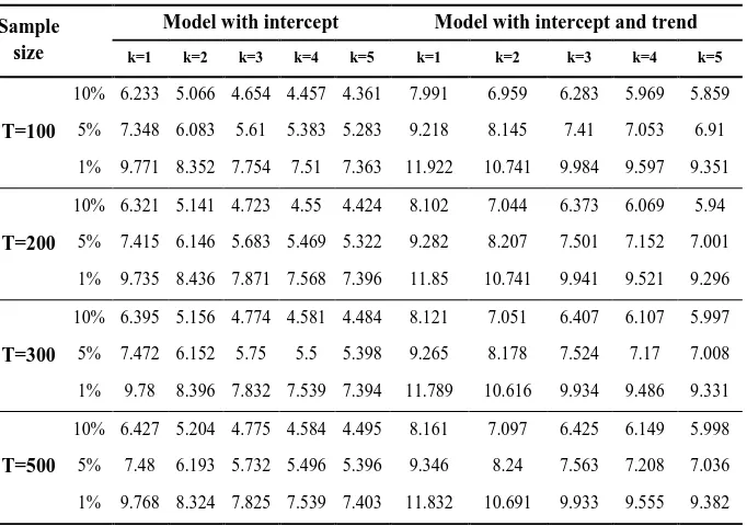
two alternative models. The first model is only assumed an intercept term in equation (2) (i.e., Z= [1]). The second model is equipped an intercept term with trend term (i.e., Z= [1,t]). With setting k between 1 to 5 and sample sizes included 100, 200, 300, and 500 observations, we compute asymptotic critical values by Monte Carlo simulation based on random walk model with pseudo-iid N(0,1) random number and 100,000 replications. The results of critical values are presented in Table 1.

Table 1: Asymptotic Critical Values

Sample size

Model with intercept Model with intercept and trend

k=1 k=2 k=3 k=4 k=5 k=1 k=2 k=3 k=4 k=5

T=100

10% 6.233 5.066 4.654 4.457 4.361 7.991 6.959 6.283 5.969 5.859 5% 7.348 6.083 5.61 5.383 5.283 9.218 8.145 7.41 7.053 6.91 1% 9.771 8.352 7.754 7.51 7.363 11.922 10.741 9.984 9.597 9.351

T=200

10% 6.321 5.141 4.723 4.55 4.424 8.102 7.044 6.373 6.069 5.94 5% 7.415 6.146 5.683 5.469 5.322 9.282 8.207 7.501 7.152 7.001 1% 9.735 8.436 7.871 7.568 7.396 11.85 10.741 9.941 9.521 9.296

T=300

10% 6.395 5.156 4.774 4.581 4.484 8.121 7.051 6.407 6.107 5.997 5% 7.472 6.152 5.75 5.5 5.398 9.265 8.178 7.524 7.17 7.008 1% 9.78 8.396 7.832 7.539 7.394 11.789 10.616 9.934 9.486 9.331

T=500

10% 6.427 5.204 4.775 4.584 4.495 8.161 7.097 6.425 6.149 5.998 5% 7.48 6.193 5.732 5.496 5.396 9.346 8.24 7.563 7.208 7.036 1% 9.768 8.324 7.825 7.539 7.403 11.832 10.691 9.933 9.555 9.382

Note: Critical values were calculated using Monte Carlo experiment based on 100,000 replications.

When the null of unit root is rejected against the alternative of stationary symmetric or asymmetric ESTAR nonlinearity, we are able to test the null hypothesis of symmetric ESTAR nonlinearity by testing H₀:₂ 0 against H₁:₂0 with a standard F-test (T-test, or Lagrange Multiplier (LM) test).

(6)

restricted unrestricted unrestricted

(SSR SSR (k )) / 2

F(k ) ,

SSR (k ) / T q

 

 



 (8)

where SSR_unrestrict_ed indicates the SSR with full regression equation (2) and SSR_restricted is the SSR without  s from short regression under the cases of with and without nonlinear component, respectively. Due to the presence of nuisance parameter, the F-test statistic has no standard distribution. We thereby employ the critical values tabulated in Becker et al. (2006).

3. Finite-Sample Size and Power Properties

3.1 Finite-Sample Size

Aiming at the test with a finite-sample size, we consider a following DGP:

* *

t t 1 2 t

t t 1 t

2 k t 2 k t

y Z sin( ) cos( ) (9)

T T

t 1, 2,..., T



 

       

     

where _t~iid(0,1) , ₁₂{0.1,1}, k* {1,2,3}, sample size } 300 , 100 { 

T , nominal size is 5%, and 10,000 replications. The values 0.1 and 1 for ₁ and ₂ are related to an almost linear and nonlinear process respectively. The results are presented in Table 2, and all reported sizes for these DGPs are close to 5%.

Table 2: Empirical Size of the Test Statistic

Model Parameter

T=100 T=300

k=1 k=2 k=3 k=1 k=2 k=3

Model with intercept 1 . 0 2 1 

 0.050 0.051 0.047 0.048 0.047 0.046

1 2 1 

 0.053 0.051 0.047 0.050 0.051 0.047

Model with intercept and trend

1 . 0 2

1 

 0.054 0.049 0.049 0.048 0.051 0.051

1 2 1 

 0.052 0.048 0.051 0.050 0.050 0.046

(7)

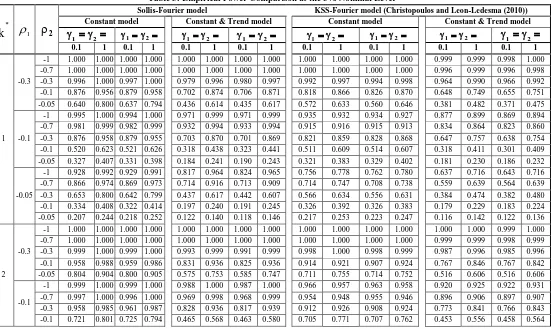
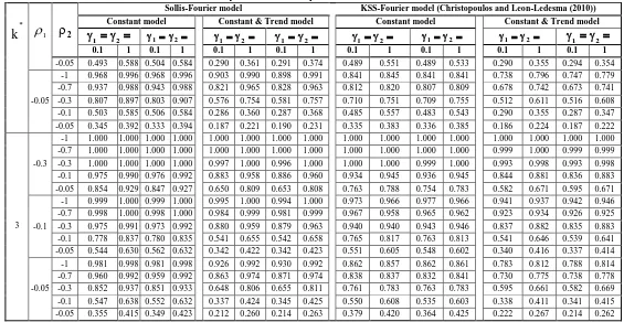
3.2. Finite-Sample Power

To investigate the finite-sample power properties from the unit root test, unlike globally stationary process, we consider a following Fourier-AESTAR model as DGP:

* *

t t 1 2 t

2

t t 1 t 1 t 1 t 2 t 1 1 t 2 t 1 2 t 1 t t

2

t 1 t 1 1 t 1 1

1

t 2 t 1 2 t 1 2

2 k t 2 k t

y Z sin( ) cos( ) (10)

T T

o o ( , o ){S ( , o ) (1 S ( , o )) }o ; ~ iid(0, )

( , o ) 1 exp( (o )) 0

S ( , o ) [1 exp( (o ))] 0

    

 



 

 

       

             

      

     

where all combinations of the parameters and frequencies values are specifiedtobethat₁{0.05,0.1,0.3},2{0.05,0.1,0.3,0.7,0.9,1},

}, 1 , 1 . 0 { 1

 ₂1, ₁₂{0.1,1}, k*{1,2,3}, ω_t~iid(0,1), and

T 300. The values 0.1 and 1 with respect to η 1 _{indicate respectively}

slow and fast transition. The small 2 corresponds to symmetric ESTAR nonlinearity, and the small 1_{linking with a big}₂_{generates the large} degree of asymmetric ESTAR nonlinearity.

(8)

In addition, the results also show that our unit root test approach is superior to the test method of Christopoulos and Leon-Ledesma (2010) for both transition parameters (i.e. slow and fast speed), and the test power increases along with the frequency.

4. Empirical Application

In this section, we employ our test statistics to re-test the RIRPH among 12 OECD countries. We extend our data set, compared with the examination of Rapach and Wohar (2004), over the period from 1960Q4 to 2012Q3. The nominal interest rate and CPI variables are collected from OECD Economic Indicators. In order to test the RIRPH, we first calculate real interest rate and further use the U.S as benchmark country to compute the real interest rate differentials series according to the following equation (11):

f f

t t t t t

(i   ) (i   ) RID (11)

(9)

(10)

*

k 1 2

Constant model Constant & Trend model Constant model Constant & Trend model

1 2

       1 2    1 2    1 2    1 2    1 2    1 2    1 2

0.1 1 0.1 1 0.1 1 0.1 1 0.1 1 0.1 1 0.1 1 0.1 1

1 -0.3

-1 1.000 _{1.000 1.000 1.000 1.000 1.000 1.000 1.000 1.000} 1.000 1.000 _{1.000 0.999} 0.999 0.998 1.000 -0.7 1.000 _{1.000 1.000 1.000 1.000 1.000 1.000 1.000 1.000} 1.000 1.000 _{1.000 0.996} 0.999 0.996 0.998 -0.3 0.996 _{1.000 0.997 1.000 0.979 0.996 0.980 0.997 0.992} 0.997 0.994 _{0.998 0.964} 0.990 0.966 0.992 -0.1 0.876 _{0.956 0.879 0.958 0.702 0.874 0.706 0.871 0.818} 0.866 0.826 _{0.870 0.648} 0.749 0.655 0.751 -0.05 0.640 _{0.800 0.637 0.794 0.436 0.614 0.435 0.617 0.572} 0.633 0.560 _{0.646 0.381} 0.482 0.371 0.475

-0.1

-1 0.995 _{1.000 0.994 1.000 0.971 0.999 0.971 0.999 0.935} 0.932 0.934 _{0.927 0.877} 0.899 0.869 0.894 -0.7 0.981 _{0.999 0.982 0.999 0.932 0.994 0.933 0.994 0.915} 0.916 0.915 _{0.913 0.834} 0.864 0.823 0.860 -0.3 0.876 _{0.958 0.879 0.955 0.703 0.870 0.701 0.869 0.821} 0.859 0.828 _{0.868 0.647} 0.757 0.638 0.754 -0.1 0.520 _{0.623 0.521 0.626 0.318 0.438 0.323 0.441 0.511} 0.609 0.514 _{0.607 0.318} 0.411 0.301 0.409 -0.05 0.327 _{0.407 0.331 0.398 0.184 0.241 0.190 0.243 0.321} 0.383 0.329 _{0.402 0.181} 0.230 0.186 0.232

-0.05

-1 0.928 _{0.992 0.929 0.991 0.817 0.964 0.824 0.965 0.756} 0.778 0.762 _{0.780 0.637} 0.716 0.643 0.716 -0.7 0.866 _{0.974 0.869 0.973 0.714 0.916 0.713 0.909 0.714} 0.747 0.708 _{0.738 0.559} 0.639 0.564 0.639 -0.3 0.653 _{0.800 0.642 0.799 0.437 0.617 0.442 0.607 0.566} 0.634 0.556 _{0.631 0.384} 0.474 0.382 0.480 -0.1 0.334 _{0.408 0.322 0.414 0.197 0.240 0.191 0.245 0.326} 0.392 0.326 _{0.383 0.179} 0.229 0.183 0.224 -0.05 0.207 _{0.244 0.218 0.252 0.122 0.140 0.118 0.146 0.217} 0.253 0.223 _{0.247 0.116} 0.142 0.122 0.136

2 -0.3

-1 1.000 _{1.000 1.000 1.000 1.000 1.000 1.000 1.000 1.000} 1.000 1.000 _{1.000 1.000} 1.000 0.999 1.000 -0.7 1.000 _{1.000 1.000 1.000 1.000 1.000 1.000 1.000 1.000} 1.000 1.000 _{1.000 0.999} 0.999 0.998 0.999 -0.3 0.999 _{1.000 0.999 1.000 0.993 0.999 0.991 0.999 0.998} 1.000 0.998 _{0.999 0.987} 0.996 0.985 0.996 -0.1 0.958 _{0.988 0.959 0.986 0.831 0.936 0.825 0.936 0.914} 0.921 0.907 _{0.924 0.767} 0.846 0.767 0.842 -0.05 0.804 _{0.904 0.800 0.905 0.575 0.753 0.585 0.747 0.711} 0.755 0.714 _{0.752 0.516} 0.606 0.516 0.606

-0.1

(11)

Table 3: Empirical Power Comparison at the 5% Nominal Level

*

k 1 2

Sollis-Fourier model KSS-Fourier model (Christopoulos and Leon-Ledesma (2010)) Constant model Constant & Trend model Constant model Constant & Trend model

1 2

       1 2    1 2    1 2    1 2    1 2    1 2    1 2

0.1 1 0.1 1 0.1 1 0.1 1 0.1 1 0.1 1 0.1 1 0.1 1

-0.05 0.493 _{0.588 0.504 0.584 0.290 0.361 0.291 0.374 0.489} 0.551 0.489 _{0.533 0.290} 0.355 0.294 0.354

-0.05

-1 0.968 _{0.996 0.968 0.996 0.903 0.990 0.898 0.991 0.841} 0.845 0.841 _{0.841 0.738} 0.796 0.747 0.779 -0.7 0.937 _{0.988 0.943 0.988 0.821 0.965 0.828 0.963 0.812} 0.820 0.807 _{0.809 0.678} 0.742 0.673 0.741 -0.3 0.807 _{0.897 0.803 0.907 0.576 0.754 0.581 0.757 0.710} 0.751 0.709 _{0.755 0.512} 0.611 0.516 0.608 -0.1 0.503 _{0.585 0.506 0.584 0.286 0.360 0.287 0.368 0.485} 0.557 0.483 _{0.543 0.290} 0.355 0.287 0.347 -0.05 0.345 _{0.392 0.333 0.394 0.187 0.221 0.190 0.231 0.335} 0.383 0.336 _{0.385 0.186} 0.224 0.187 0.222

3 -0.3

-1 1.000 _{1.000 1.000 1.000 1.000 1.000 1.000 1.000 1.000} 1.000 1.000 _{1.000 1.000} 1.000 1.000 1.000 -0.7 1.000 _{1.000 1.000 1.000 1.000 1.000 1.000 1.000 1.000} 1.000 1.000 _{1.000 0.999} 1.000 0.999 0.999 -0.3 1.000 _{1.000 1.000 1.000 0.997 1.000 0.996 1.000 1.000} 1.000 0.999 _{1.000 0.993} 0.998 0.993 0.998 -0.1 0.975 _{0.990 0.976 0.992 0.883 0.958 0.886 0.960 0.934} 0.945 0.936 _{0.945 0.844} 0.881 0.836 0.883 -0.05 0.854 _{0.929 0.847 0.927 0.650 0.809 0.653 0.808 0.763} 0.788 0.754 _{0.783 0.582} 0.671 0.595 0.671

-0.1

-1 0.999 _{1.000 0.999 1.000 0.995 1.000 0.994 1.000 0.973} 0.966 0.977 _{0.966 0.941} 0.937 0.942 0.946 -0.7 0.998 _{1.000 0.998 1.000 0.984 0.999 0.981 0.999 0.967} 0.958 0.965 _{0.962 0.923} 0.934 0.926 0.925 -0.3 0.975 _{0.991 0.973 0.992 0.880 0.959 0.879 0.963 0.940} 0.940 0.943 _{0.946 0.837} 0.882 0.835 0.883 -0.1 0.778 _{0.837 0.780 0.835 0.541 0.655 0.542 0.658 0.765} 0.817 0.763 _{0.813 0.541} 0.646 0.539 0.641 -0.05 0.544 _{0.630 0.562 0.632 0.342 0.422 0.342 0.423 0.551} 0.605 0.548 _{0.602 0.340} 0.416 0.337 0.414

-0.05

-1 0.981 _{0.998 0.981 0.998 0.926 0.992 0.930 0.992 0.862} 0.857 0.862 _{0.861 0.783} 0.812 0.788 0.814 -0.7 0.960 _{0.992 0.959 0.992 0.863 0.974 0.871 0.974 0.838} 0.837 0.832 _{0.841 0.730} 0.775 0.738 0.778 -0.3 0.852 _{0.937 0.851 0.933 0.648 0.806 0.655 0.811 0.761} 0.783 0.763 _{0.783 0.595} 0.661 0.582 0.669 -0.1 0.547 _{0.638 0.552 0.632 0.337 0.424 0.345 0.425 0.550} 0.608 0.535 _{0.603 0.338} 0.411 0.341 0.415 -0.05 0.355 _{0.415 0.349 0.423 0.212 0.260 0.214 0.263 0.379} 0.420 0.364 _{0.425 0.222} 0.267 0.214 0.262

(12)

(13)

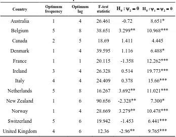
Table 4: Empirical Results for RIRPH

Country Optimum frequency

Optimum lag

F-test

statistic H :0  2 0 H :0    1 2 0

Australia 1 4 26.461 -0.72 8.651*

Belgium 5 8 38.651 3.299** 10.968***

Canada 2 5 18.69 1.411 4.445

Denmark 1 4 39.595 1.116 6.488*

France 1 1 20.115 -1.358 12.262***

Ireland 3 4 26.328 0.514 19.773***

Italy 4 4 24.409 0.378 15.66***

Netherlands 5 8 16.267 3.692** 11.021***

New Zealand 1 6 90.656 -2.328** 7.300*

Norway 1 4 28.669 3.279** 10.478***

Switzerland 5 6 19.942 -1.453 6.441***

United Kingdom 4 6 12.36 -2.96** 9.765***

Note: The optimum lag order selected based on the recursive t-statistic. ***, ** and * indicate the null hypothesis is rejected at the 1%, 5% and 10% levels, respectively.

5. Conclusion

In this paper, we generalize the Sollis (2009) AESTAR nonlinear unit root test with allowing multiple smooth temporary breaks by calculating means in Fourier function. The simulation results of Monte Carlo studies also show that our empirical test approach is more reliable and its test statistic is much powerful. Lastly, we further employ our test to examine the real interest rate parity hypothesis over 12 OECD countries and find that the RID series are short-lived, nonlinear mean reversing with multiple smooth breaks, and some adjustments deviated from equilibrium are asymmetrical.

References

(14)

Becker, R., Enders, W., & Lee, J. (2004). A General Test for Time Dependence in Parameters. Journal of Applied Econometrics, 19, 899–906.

Becker, R., Enders, W., & Lee, J. (2006). A Stationary Test in the Presence of an Unknown Number of Smooth Breaks. Journal of Time Series Analysis,27, 381–409.

Christopoulos, D. K., & Leon-Ledesma, M. A. (2010). Smooth Breaks and Non-Linear Mean Reversion: Post-Bretton Woods Real Exchange Rates. Journal of International Money and Finance, 29, 1076–1093.

Enders, W., & Lee, J. (2012). A Unit Root Test Using a Fourier Series to Approximate Smooth Breaks. Oxford Bulletin of Economics and Statistics,74(4), 574–599.

Gallant, R. (1981). On the Basis in Flexible Functional Form and an Essentially Unbiased Form: The Flexible Fourier Form. Journal of

Econometrics,15, 211–353.

Rapach, D. E., & Wohar, M. E. (2004). The Persistence in International Real Interest Rates. International Journal of Finance

and Economics,9, 339–346.