in the population sciences published by the Max Planck Institute for Demographic Research Konrad-Zuse Str. 1, D-18057 Rostock · GERMANY www.demographic-research.org
DEMOGRAPHIC RESEARCH
VOLUME 22, ARTICLE 6, PAGES 129-158
PUBLISHED 26 JANUARY 2010
http://www.demographic-research.org/Volumes/Vol22/6/ DOI: 10.4054/DemRes.2010.22.6
Research Material
Estimation of multi-state life table functions
and their variability from complex survey
data using the SPACE Program
Liming Cai
Mark D. Hayward
Yasuhiko Saito
James Lubitz
Aaron Hagedorn
Eileen Crimmins
© 2010 Liming Cai et al.
This open-access work is published under the terms of the Creative Commons Attribution NonCommercial License 2.0 Germany, which permits use, reproduction & distribution in any medium for non-commercial purposes, provided the original author(s) and source are given credit.
1 Introduction 130
2 The SPACE Program 132
2.1 The MSLT Model 132
2.2 Data 134
2.3 Estimation algorithms for model parameters 135 2.4 Micro-simulation and bootstrapping 136 2.5 Comparison of SPACE with IMaCh and GSMLT 138
2.6 Application 139
2.6.1 Comparison of IMaCh and SPACE estimates 140 2.6.2 Convergence of bootstrap variance estimates 144 2.6.3 The distribution of years lived and spent in different health states 147
3 Discussion and conclusion 150
4 Acknowledgements 152
Estimation of multi-state life table functions and their variability
from complex survey data using the SPACE Program
1Liming Cai2
Mark D. Hayward3
Yasuhiko Saito4 James Lubitz5
Aaron Hagedorn6
Eileen Crimmins7
Abstract
The multistate life table (MSLT) model is an important demographic method to document life cycle processes. In this paper, we present the SPACE (Stochastic Population Analysis for Complex Events) program to estimate MSLT functions and their sampling variability. It has several advantages over other programs, including the use of micro-simulation and the bootstrap method to estimate the variance of MSLT functions. Simulation enables researchers to analyze a broader array of statistics than the deterministic approach, and may be especially advantageous in investigating distributions of MSLT functions. The bootstrap method takes sample design into account to correct the potential bias in variance estimates.
1 Disclaimer: The findings and conclusions in this paper are those of the author(s) and do not necessarily
represent the views of the National Center for Health Statistics, Centers for Disease Control and Prevention.
2 Office of Analysis and Epidemiology, National Center for Health Statistics. 3311 Toledo Road, room 6330,
Hyattsville, MD 20782; email: [email protected]; tel: 301-458-4133.
3 Population Research Center and Department of Sociology, University of Texas at Austin. 4 Advanced Research Institute for the Sciences and Humanities, Nihon University, Japan. 5 Office of Analysis and Epidemiology, National Center for Health Statistics.
1. Introduction
The multi-state life table (MSLT) model is a “time-inhomogeneous, finite-space, continuous-time” Markov model (Schoen 1988:64). Demographers frequently use it to analyze stochastic processes involving multiple and recurrent events to estimate expected duration in various states: for example functional limitations (Crimmins, Hayward, and Saito 1994, 1996; Land, Guralnik, and Blazer 1994); HIV/AIDS (Palloni 1996)’ labor force participation (Hayward and Grady 1990; Hayward, Grady, and McLaughlin 1988): cohabitation and marriage (Bumpass and Lu 2000; Espenshade and Braun 1982; Hofferth 1985; Schoen and Land 1979): poverty (Duncan and Rodgers 1988): and living in socio-economically disadvantaged neighborhoods (Quillian 2003). It has also been used in studies linking longevity to medical spending for the aging population (Goldman et al. 2005; Lubitz et al. 2003).
When the MSLT model was originally developed, life tables were calculated using population-level rates – hence there was limited attention given to estimation techniques and variability in the life table functions. Increasingly, however, the data source is panel data obtained via survey sampling, making it difficult to obtain reliable estimates of life table inputs (i.e., transition rates or probabilities) directly from raw data (Saito, Crimmins, and Hayward 1991). As a result, regression models are used to produce smoothed estimates of life table input, and the variance of MSLT functions is now needed to test hypotheses about the differences between population subgroups.
Currently there are two programs that are publicly available to perform these tasks – the IMaCh (Interpolated Markov Chain) program and the GSMLT (Gibbs Sampling Multistate Life Table) program.8 The IMaCh program is introduced by Lièvre, Brouard
and, Heathcote (2003). It estimates transition probabilities using a discrete-time “embedded” Markov chain (eMC) approach, developed by Laditka and Wolf (1998).9
The eMC approach, in contrast to the traditional event history approach, recognizes that observed sample data often fail to include many events of short duration between infrequent follow-up interviews (Hardy and Gill 2004). To recover these missing events, the eMC approach applies the MSLT model to shorter transition periods (e.g., monthly, quarterly, etc.) that are “embedded” within the longer interval between follow-ups. The variance of MSLT functions is estimated as a linear function of the variance and covariance of transition probabilities using the Delta method. Currently, the IMaCh
8 There is another publically available program to estimate MSLT health expectancy (Weden 2005,
downloadable from http://www.ssc.wisc.edu/~mweden/). Since this program does not estimate the sampling variability of MSLT functions, we will not discuss it here.
9 Land, Guralnik, and Blazer (1994) developed a continuous-time Markov process model with
program can estimate health expectancy (HE) and “equilibrium” prevalence of health states (i.e., implied by transition probability estimates in a stationary population), and their variances. The GSMLT program is introduced in Lynch and Brown (2005) and takes a Bayesian approach to estimating life table quantities. In its Bayesian framework, transition probabilities are estimated using a constrained discrete-time multinomial probit model (Lynch and Brown 2005). Once the iterative algorithm has converged, it draws a large number of samples from the posterior distribution of transition probabilities to generate for each sample a multi-state life table, from which the posterior distribution of life table functions can be obtained. The posterior distribution allows researchers to obtain estimates on a range of distributional statistics, including their means and variances. Currently, the GSMLT program only estimates HE and its variance.
This paper introduces another program – the SPACE (Stochastic Population Analysis for Complex Events) program. While the MSLT model fitted in the SPACE program takes the traditional event history approach (i.e., assuming no missing events of short duration between successive interviews), it has two analytical advantages over the other two programs. First, the SPACE program uses micro-simulation to estimate MSLT functions. Micro-simulation is an increasingly popular computational tool in demography research (e.g., Cai and Lubitz 2007; Cai, Schenker, and Lubitz 2006; Laditka et al. 2007; Laditka and Wolf 1998; Lubitz et al. 2003; Wolf 1986; Wolf, Laditka, and Laditka 2002). It “expresses” the transition probability estimates by generating detailed life paths for each member of the target population. As a result, the SPACE program allows users to estimate a variety of MSLT functions directly from simulated data. This computational flexibility compares favorably to the rigidness of the deterministic approach used in the IMaCh program where only a limited number of summary statistics can be produced.
stratification and multi-stage clustering, which, if not adequately controlled for, will result in biased variance estimates and invalid statistical inference (Lohr 1999).
In the following sections, we will discuss the details of the SPACE program and present some results from an application of the SPACE program to highlight its differences from the IMaCh program and to demonstrate its usefulness. We chose to compare the estimates, by gender and race/ethnicity, with the IMaCh program because it is relatively easy to implement and widely used. The SPACE program is currently available upon request from the authors, and will be available for download from REVES (http://reves.site.ined.fr/en/resources/computation_online/).
2. The SPACE Program
The SPACE program is a statistical program developed to estimate the MSLT functions from survey data. It consists of multiple sets of PC-based SAS® programs with different
modeling capacity. However, they are structured similarly: each set of the program contains two components – the data component and the statistical component. The data component prepares the input data sets – both for the full analysis sample and for the bootstrap samples drawn from the full sample – for the statistical component. The statistical component estimates transition rates or probabilities and the MSLT functions based on the estimated parameters. The output includes estimates of MSLT functions and their variances.
2.1 The MSLT Model
The MSLT model characterizes population movement over time in a finite, discrete and mutually exclusive state space as a Markov process. Two types of MSLT models can be fitted in the SPACE program: one follows a first-order Markov chain where the transition probabilities are conditional only on the current age and status, and another follows a semi-Markov process (SMP) model where the transition probabilities are age, status and duration dependent. Since we compare to the IMaCh estimates in this study, we will only consider the duration-independent MSLT model in detail here.
restrictive, as spells of short durations may occur frequently between interviews (Hardy et al. 2005). As interviews become less frequent (e.g., every five years), the number of events that the model fails to capture are likely to rise and additional bias can be introduced into the estimates of MSLT functions (Gill et al. 2005; Wolf and Gill 2009)
The SPACE program uses a class of discrete-time hazard models to estimate the age-specific transition probabilities or rates from sample data. The SPACE program can fit a multinomial logistic regression as in Laditka and Wolf (1998) to estimate the transition probabilities directly. The equation takes the following basic form:
, ) ) , ( ) , (
log( a b age c othercovariates t age p t age p ij t ij ij ii
ij = + ∗ + ∗ (1)
where is the transition probability from the current state i to state ( ) over the annual interval at
) ,t age j i n j
i, =1,2,3,..., , ≠ aij
ij (
pij
j aget, is the intercept, and is
the coefficient for age at the beginning of annual interval, and c is the set of coefficients for other covariates.
ij b
Alternatively, the SPACE program can estimate the transition rates as in Hayward and Grady (1990) and Crimmins, Hayward, and Saito (1994). The model takes the
following form:
, )
, (
logµij aget =aij+bij∗aget+cij∗othercovariates (2)
ij µ
where is the instantaneous transition rates from current state i to state ( ) over the annual interval at . The transition rates are converted into transition probabilities using the formula in Crimmins, Hayward, and Saito (1994:165).
j ≠ j
i n j
i, =1,2,3,..., , aget
The SPACE program imposes no limit on the number of non-absorbing states in the MSLT models; the number of states depends only on the data and research objective. Also, multiple categorical covariates measured at study baseline (e.g., gender, race/ethnicity, education, etc.) can be included. These covariates may each have more than two categories and their values remain fixed during the survey period.10 Finally,
the SPACE program permits uneven lengths in observation intervals, which are calculated as the number of years between interviews.11 The program converts input
data from person-year format to annual interval format in which each line of data
10 Time-dependent covariates can be incorporated into MSLT models as in Yang and Hall (2008). Future
versions of SPACE will address this issue.
11 Currently the SPACE program estimates transition parameters over annual transition intervals. If the input
represents the movement from one interview to the next over the period of one year. If the length of the interval between interviews is two or more years, then a corresponding number of annual intervals are created to facilitate the computation of annual transition parameters. The events are assumed to occur randomly in one of these annual intervals. This approach results in the events occurring, on average, in the middle of the observation interval.
The outputs of these regressions are age-specific transition probability estimates for all possible transitions, conditional on the other covariates included in the model. The SPACE program provides two options to estimate MSLT functions: the deterministic approach as in IMaCh or GSMLT or micro-simulation. The deterministic approach can only estimate HE, while micro-simulation can be used to estimate HE and a variety of other MSLT functions. The details of micro-simulation are discussed in section 2.4.
2.2 Data
The study population for this analysis is drawn from the 1998-2002 panels of the Medicare Current Beneficiary Survey (MCBS). The MCBS is a nationally representative, multi-stage, longitudinal panel survey of the Medicare population, sponsored by the Centers for Medicare and Medicaid Services (CMS), and conducted continuously since 1991. The survey gathers data on a wide range of topics including health status, socio-demographic information, and the use and cost of medical services. Survey records are linked to administrative data on use of and expenditures on Medicare-covered services (hospital, physician, etc.) and on vital status.
The MCBS follows a rotating panel design. Each year a new panel that is representative of the current Medicare population is selected from the list of eligible beneficiaries. Each person in the panel is scheduled to receive 12 interviews over a four-year period, with information on self-reported health status collected once a year in the Fall. The panel is not renewed during the four-year period, but the rates of attrition are small and decline over time. Given the adjustment for survey non-response in sample weights, the bias in estimates is substantially reduced or eliminated (Kautter et al. 2006).
are selected. The analysis sample used in this study has a total of 112 strata and 1,168 PSUs. The individual Medicare beneficiaries are then selected in the third stage (i.e., within each zip-code cluster) stratified by seven age groups (under 45, 45 to 64, 65 to 69, 70 to 74, 75 to 79, 80 to 84 and 85 and over). The oldest people (85 and over) and disabled people (64 and under) are oversampled to allow detailed analysis of their health status and health care needs.
For this study, we use the 1998-2002 panels that contain 14,892 elderly beneficiaries. We exclude 1,017 persons of Hispanic origin or other racial/ethnic groups to focus on non-Hispanic whites and blacks only, since the IMaCh program does not accept more than two categories at a time for any covariate. The full analysis sample contains 50,830 person-year observations for 13,875 persons of age 65 and older.
) 1
2 (i=
) 3
=
i
For explication purposes, we use a simple dichotomous measure of health based only on the presence of limitations in activities of daily living (ADLs). A person is considered disabled ( if he or she either responds “yes” to having difficulty with one or more of the six ADLs (bathing, dressing, eating, transferring, walking, and using the toilet), or responds “does not do the activity because of a health or physical problem.” Otherwise, this person is considered non-disabled or ‘active’ . For those who report limitations with any of the activities, the survey also asks whether they receive help from another person and/or use special equipment. We do not consider “receiving help” in defining functional disability in this study. Survey respondents can move between the disabled and non-disabled states over time; while ‘dead’ ( is an absorbing state.
=
i
)
2.3 Estimation algorithms for model parameters
The regressions specified above are carried out by two SAS procedures: PROC LOGISTIC and PROC LIFEREG. These procedures offer powerful modeling capabilities. For example, users can use the current state as one of the covariates, instead of using it to stratify the data. Users can select the best functional form for the whole sample, or choose different forms for subsets of the data.12 They can also relax
the linear relationship between age and the logit to test other functional forms (e.g., logarithm or polynomial functions), or even to evaluate different forms of the link function (e.g., cumulative, multinomial or complementary log-log). This degree of flexibility is not available in the IMaCh and GSMLT programs.
12 When sample data are drawn from complex surveys, variable selection should be carried out using
2.4 Micro-simulation and bootstrapping
Micro-simulation is the main computation technique used by the SPACE program to estimate MSLT functions. Compared to the deterministic approach, micro-simulation holds substantial advantages in terms of the scope of statistics one can calculate. With the deterministic approach, one essentially moves the entire population through the transition matrices, with little insight into individual dynamics. As a result, only a few summary statistics can be derived. Micro-simulation, however, simulates the life path of all members of the population such that a wide variety of summary statistics of the population dynamics can be derived.
The population simulated in the SPACE program is not arbitrary. It is characterized by the estimated transition parameters, conditional on the covariates included in the regression models. To briefly describe how it works, suppose we want to simulate the life histories of a 100,000-person cohort of 65-year old black men. For a hypothetical member of this cohort, we first randomly assign an initial health status, say, active, at age 65 based on the weighted health distribution for black men at age 65 from the input data. We then evaluate possible health changes between age 65 and 66 by comparing a random number from the uniform distribution with the transition probabilities for the age 65-66 interval, given his current status of active health. If his health status changes to disabled, then we generate a new random number from the uniform distribution to compare with the transition probabilities for the age 66-67 interval, conditional on being disabled at age 66. The result of this comparison determines if his health status changes again between age 66 and 67, and is repeated one year at a time until his eventual death. Once this process is repeated for all members of the cohort, we have a complete record of individual health histories from which MSLT functions can be easily calculated by averaging over the individual records. For example, total life expectancy (TLE) is computed by the average number of years lived for the simulated 100,000-person cohort. HE, including expected length of time spent in both active health (ALE) and disability (DLE), is computed by the average number of years spent in each health state.
It is worth noting that the simulation is based upon parameters of a period life table, where the experience of an eighty-year old today is assumed to hold for the next twenty years when a current sixty-year old reaches his or her eightieth birthday. This is unlikely to be the actual experience of any individual. Therefore, the simulated life paths should not be regarded as the actual experience of a single cohort over time.
one wants to test the hypothesis that males and females differ in their expected health over the life cycle (i.e. expected years in various health states). Health expectancy is determined by age-specific rates of movement into and out of the health states, including the risk of death from each health state. How sex is associated with health expectancy, however, may be unclear for a number of reasons. Sex may significantly affect some transitions and not others. Or, sex effects, even though statistically significant, may be offsetting. It is also possible that sex effects may be non-significant for the whole set of transitions, yet the consistency of effects for a lengthy period of time may combine in a way in which the sex effects are reinforced and magnified with age. The hypothesis of sex differences in health is therefore global in the sense that it takes into account sex differences in all of the transitions defining the process of life cycle health.
In addition, variance estimation for a complex survey needs to consider sources of variability due to stratification and multi-stage clustering that are not present in a simple random sample (SRS). Treating a stratified sample as a SRS usually overestimates the variance, while treating a clustered sample as SRS usually underestimates the variance. Although the net effect is often not obvious, it is nonetheless clear that ignoring the complex sampling design can lead to incorrect statistical inference (Lohr 1999).
1
−
h
n h h
h h
To address these issues, the SPACE program uses a version of the rescaling bootstrap method developed specifically for complex surveys (Korn and Graubard 1999:32-33; Rao and Wu 1988; Sitter 1992a), and which has been implemented in recent demographic studies (e.g., Cai and Lubitz 2007; Cai et al. 2006). This approach samples PSUs with replacement within the stratum , where n is the number of PSUs in stratum . For each PSUi sampled from stratum , the original sample weight
is multiplied by *mi i
h h
n n
1
− , where m is the number of times the PSUi is selected. If a rare event is not represented in a particular bootstrap sample, the sample can be redrawn.
sampling fraction, which is typically not available to researchers using the public versions of the survey data.
The bootstrap method usually requires more computation, and its theoretical properties in complex surveys are not fully studied (Lohr 1999). There is also evidence from simulation studies that the bootstrap method may not outperform the Jackknife and the Balanced Repeated Replication (BRR) methods for stratified one-stage SRS with replacement (Kovar, Rao, and Wu 1988). But, the bootstrap method also has a number of advantages. It can be used to estimate the variance for a broader class of statistics, including sample quantiles. It can also provide consistent variance estimators for surveys with imputed data, and has a “higher potential to be extended to other complex problems” than the BRR and jackknife approaches (Shao and Tu 1995:280). From a practitioner’s perspective, it is reasonable to conclude that the bootstrap method is a suitable all-purpose variance estimator for MSLT functions.
2.5 Comparison of SPACE with IMaCh and GSMLT
There are several major differences among the three programs. The first is their assumptions about the “completeness” of observed data. The IMaCh program takes the eMC approach assuming that observed data are incomplete and allows multiple events between successive interviews. The SPACE and GSMLT program, on the other hand, takes the traditional event history approach assuming that the observed data are complete and allows only one (or zero) event between successive observations. Although the assumption of eMC is conceptually more realistic, a recent study shows that the estimates of HE and transition probabilities from both approaches are surprisingly similar – both are biased (Wolf and Gill 2009). Since HE estimates may be insensitive to the length of the interval between interviews for up to two years (Gill et al. 2005), it is possible that estimates based on both approaches become more biased as the interview becomes less frequent.
Another difference lies in their treatment of the design factors of the survey data. Currently, the GSMLT program makes no adjustment for survey design and assumes input data are from a SRS, while the IMaCh program makes only limited adjustment by assuming that the survey design affects only the sample weight. Since the sample weight reflects the probability of the selection of individuals, not clusters, it cannot remove the bias in variance estimates in clustered survey data (Lohr 1999).
estimates MSLT functions that can be expressed as a function of the transition probabilities, many statistics that may be of interest to researchers do not meet this criteria (e.g., the probability of death within two years after two prior episodes of disability, or the median of healthy life years). In addition, the complexity of expressing the mathematical relation of MSLT functions to transition probabilities may be challenging for many users.
2.6 Application
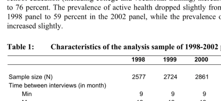
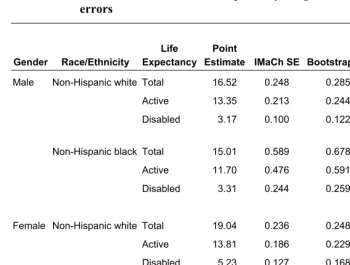
In this section we will present the results from an application of the SPACE program and compare them to the IMaCh program. Table 1 shows selected characteristics of sampled persons in the study population. The majority of sampled persons are female, non-Hispanic, white, and between the ages of 65 and 74 and free of ADL limitations. The educational achievement of the panels shows some improvement between 1998 and 2002. The proportion with less than a high school education dropped from 29 percent to 24 percent, while the proportion of high school graduates and those with more than high school education (including college and vocational training) increased from 71 percent to 76 percent. The prevalence of active health dropped slightly from 62 percent in the 1998 panel to 59 percent in the 2002 panel, while the prevalence of ADL limitations increased slightly.
Table 1: Characteristics of the analysis sample of 1998-2002 panels in MCBS
1998 1999 2000 2001 2002
Sample size (N) 2577 2724 2861 2882 2831 Time between interviews (in month)
Min 9 9 9 8 8
Mean 12 12 12 12 12
Max 16 16 16 16 16
(in weighted percents of sample size)
Gender
Male 40.3 40.4 42.3 41.4 41.8
Female 59.7 59.7 57.7 58.7 58.2
Race/Ethnicity
Table 1: (Continued)
1998 1999 2000 2001 2002 Age
65-74 57.9 56.5 54.7 53.0 53.7
75-84 32.4 33.8 35.4 35.4 34.4
85+ 9.7 9.7 9.9 11.7 11.9
Education*
Less than high school - 29.0 27.7 26.9 23.6 High school graduates - 29.7 29.4 30.9 33.8 More than high school - 41.3 42.9 42.2 42.7 Functional status at first interview
Active (no ADL limitation) 73.5 72.0 70.9 72.0 72.0 Disabled (1+ADL limitation) 26.5 28.0 29.1 28.0 28.0
Note: ADL stands for Activities of Daily Living.
*: Starting in 1999, the question on education changed to reflect the highest degree achieved, rather than the number of years in school. Therefore we suppress the estimates for 1998 to facilitate comparisons.
2.6.1 Comparison of IMaCh and SPACE estimates
The coefficient estimates of the logistic regressions from both programs are shown in Tables 2A. We fit the same logistic regressions of the form of eq. (1) for both the IMaCh and SPACE programs. In Table 2A, the IMaCh coefficients are estimated with both one-month and 12-month transition intervals, and the SPACE coefficients are estimated with an annual interval. For both programs, the gender coefficients indicate that elderly women are more likely than elderly men to become disabled, while less likely to recover and to die. The race/ethnicity coefficients indicate that elderly non-Hispanic blacks are more likely to become disabled and die, while less likely than elderly non-Hispanic whites to recover from disability.
Table 2A: Logistic regression coefficients to calculate MSLT transition probabilities in the IMaCh and SPACE program
IMaCh – Monthly Interval
Current State Destination State Intercept Age (in yrs) Female Non-Hisp Black Active Disabled -9.1406 0.0619 0.1795 0.1893 Active Death -12.8755 0.0856 -0.5982 0.2458 Disabled Active 0.8304 -0.0550 -0.1152 -0.0885 Disabled Death -9.3780 0.0677 -0.5077 0.0399
IMaCh – 12-month Interval
Current State Destination State Intercept Age (in yrs) Female Non-Hisp Black Active Disabled -7.5114 0.0709 0.2413 0.2121 Active Death -11.6119 0.1085 -0.4705 0.3249 Disabled Active 4.3619 -0.0661 -0.1940 -0.1379 Disabled Death -6.6670 0.0690 -0.5892 0.0099
SPACE – Annual Interval
Current State Destination State Intercept Age (in yrs) Female Non-Hisp Black Active Disabled -7.3928 0.0694 0.2512 0.2111 Active Death -11.2588 0.1057 -0.4657 0.3014 Disabled Active 4.3649 -0.0661 -0.1971 -0.1360 Disabled Death -6.7215 0.0702 -0.5842 0.0208
Source: The 1998-2002 Medicare Current Beneficiary Survey.
Note: Men and non-Hispanic whites are the reference categories of gender and race, respectively. All coefficients are significant at the 5 percent level.
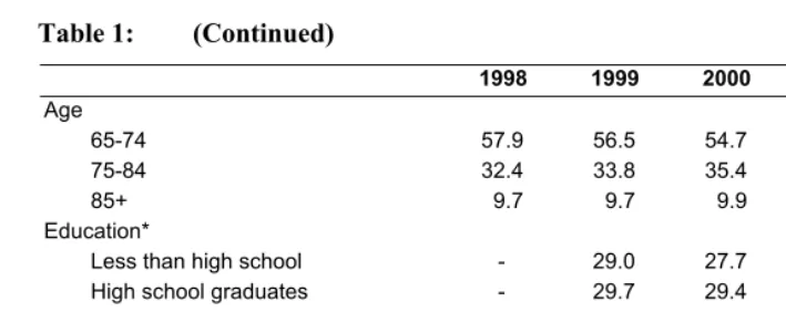
Table 2B: Observed and estimated prevalence of health status as input to the IMaCh and SPACE program, in percents
IMaCh - Period Prevalence Monthly Annual Gender Race/ Ethnicity Status
at Age 65
Observed Prevalence
Interval
SPACE - Predicted Prevalence
Male Non-Hispanic white Active 85.84 92.48 92.25 89.16 Disabled 14.16 7.52 7.75 10.84
Male Non-Hispanic black Active 87.96 90.13 89.65 86.27 Disabled 12.04 9.87 10.35 13.73
Female Non-Hispanic white Active 83.12 90.47 90.20 85.73 Disabled 16.88 9.53 9.80 14.27
Female Non-Hispanic black Active 79.39 87.55 86.95 77.95
Disabled 20.61 12.45 13.05 22.05
Source: The 1998-2002 Medicare Current Beneficiary Survey.
Note: The IMaCh period prevalence is the equilibrium prevalence in a stable population. Due to the small sample size of 65- year olds in MCBS, the observed prevalence is based on the average prevalence of 65- and 66-year olds.
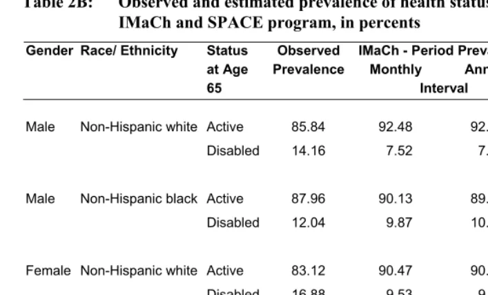
Using the IMaCh estimates of coefficients with monthly transition interval in Table 2A and the period prevalence estimates in Table 2B, the IMaCh estimates of HE at age 65 by gender and race/ethnicity are shown in Table 3. We also include in Table 3 two sets of variance estimates – the bootstrap estimates that consider survey design and the IMaCh estimates that do not – in order to evaluate the degree of bias in variance estimates when complex survey design is ignored. The bootstrap variance estimates are obtained by first randomly selecting 250 bootstrap samples from the full analytic sample, and then using them as input data sets to the IMaCh program to derive 250 sets of IMaCh point estimates of life expectancy.13 The standard deviation of these 250 estimates are considered the bootstrap SEs of the original IMaCh point estimates and are compared to the IMaCh estimates that do not reflect the complex sampling design of MCBS.
13 We also examined the variance estimates from 500 bootstrap samples and found only small differences
Table 3: IMaCh estimates of health expectancy at age 65 and their standard errors
DEFF
Gender Race/Ethnicity Life Expectancy
Point
Estimate IMaCh SE Bootstrap SE
=
) ) IMaCh Bootstrap var( var(
Male Non-Hispanic white Total 16.52 0.248 0.285 1.32
Active 13.35 0.213 0.244 1.31
Disabled 3.17 0.100 0.122 1.49
Non-Hispanic black Total 15.01 0.589 0.678 1.33
Active 11.70 0.476 0.591 1.54
Disabled 3.31 0.244 0.259 1.13
Female Non-Hispanic white Total 19.04 0.236 0.248 1.10
Active 13.81 0.186 0.229 1.52
Disabled 5.23 0.127 0.168 1.75
Non-Hispanic black Total 17.58 0.546 0.641 1.38
Active 12.11 0.434 0.550 1.61
Disabled 5.47 0.324 0.327 1.02
Source: IMaCh estimates from the 1998-2002 Medicare Current Beneficiary Survey, assuming monthly transition intervals. Bootstrap standard errors are the standard deviations of 250 bootstrap estimates.
2.6.2 Convergence of bootstrap variance estimates
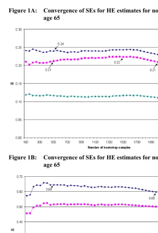
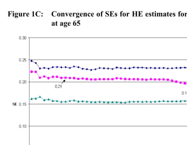
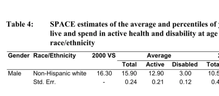
A practical issue in the implementation of bootstrap method is how many bootstrap samples to draw. Efron (1987) suggested that 100 samples are sufficient for variance estimates, while other researchers have argued for a much higher number of replications, especially given the rapidly declining cost of computation (e.g., Booth and Sarkar 1998; Chernick 1999). From a practitioner’s perspective, a straightforward approach is to check the convergence pattern of bootstrap variance estimates as more and more samples are drawn. The analyst can typically decide on the number of samples to draw when the variance estimates begin to stabilize. In Figures 1A-1D, we plot the standard errors (SEs) for SPACE estimates of HE at age 65. While the patterns are different across gender and racial/ethnic groups, all four figures show that the SEs begin to stabilize after the first 500 samples. The fluctuations after 500 samples are very small, except maybe for the TLE estimates for 65-year old black men and black women. The SEs for these two groups are 0.60 and 0.52 with 2000 samples, representing a small difference of six and seven percent, respectively, from their corresponding values with 500 samples. The convergence patterns for the percentile estimates of years lived and spent in active health and disability are similar to Figures 1A-1D and not shown here. Since these small differences are not likely to affect the results of hypothesis tests, we choose to use the SEs with 500 bootstrap samples in Table 4.14
14 The convergence patterns for the SEs in Table 4 are different from the SEs in Table 3. This is likely the
Figure 1A: Convergence of SEs for HE estimates for non-Hispanuc white men at age 65
Figure 1C: Convergence of SEs for HE estimates for non-Hispanic white women at age 65
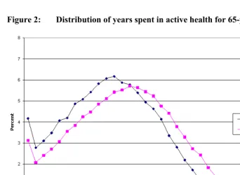
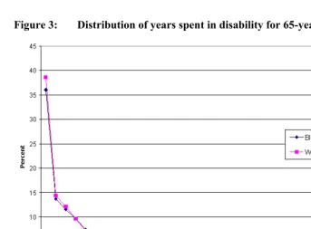
2.6.3 The distribution of years lived and spent in different health states
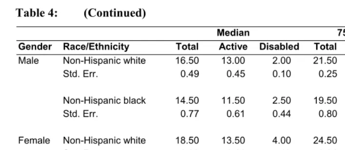
Table 4 shows the SPACE estimates of the average, median, 25th and 75th percentiles of
the number of years lived, as well as the number of years spent in active health and disability at age 65, by gender and race/ethnicity, based on transition probabilities and prevalence estimated from the full analysis sample as shown in Table 2A and 2B. We also include the TLE at age 65 based on the National Vital Statistics System in 2000 as a comparison (Arias 2002). The SPACE estimates of TLE in Table 4 indicate some small differences from the 2000 Vital Statistics: the largest is 4.7 percent for white women. The differences are caused mostly by the lack of control for variation in the actual time interval between interviews in the SPACE program. We verified this source of difference by manually calculating the transition probabilities using the SPACE coefficient estimates and the IMaCh coefficient estimates with a 12-month transition interval in Table 2A. The IMaCh estimates of TLE with a 12-month interval are closer to the Vital Statistics in year 2000 than the SPACE estimates.
Table 4: SPACE estimates of the average and percentiles of years expected to
live and spend in active health and disability at age 65, by gender and race/ethnicity
Gender Race/Ethnicity 2000 VS Average 25th Percentile
Total Active Disabled Total Active Disabled Male Non-Hispanic white 16.30 15.90 12.90 3.00 10.50 8.50 1.00
Std. Err. - 0.24 0.21 0.12 0.43 0.42 0.13
Non-Hispanic black 14.50 14.50 11.30 3.20 8.50 6.50 1.00 Std. Err. - 0.64 0.51 0.26 0.70 0.52 0.25
Female Non-Hispanic white 19.20 18.30 13.40 5.00 12.50 8.50 2.00 Std. Err. - 0.23 0.21 0.16 0.34 0.40 0.21
Table 4: (Continued)
Median 75th Percentile
Gender Race/Ethnicity Total Active Disabled Total Active Disabled Male Non-Hispanic white 16.50 13.00 2.00 21.50 17.50 4.50
Std. Err. 0.49 0.45 0.10 0.25 0.18 0.42
Non-Hispanic black 14.50 11.50 2.50 19.50 15.50 5.00
Std. Err. 0.77 0.61 0.44 0.80 0.67 0.40
Female Non-Hispanic white 18.50 13.50 4.00 24.50 17.50 7.00
Std. Err. 0.33 0.18 0.09 0.31 0.34 0.35
Non-Hispanic black 17.50 11.50 4.50 22.50 15.50 8.00
Std. Err. 0.69 0.54 0.44 0.70 0.57 0.55
Source: SPACE estimates are derived from micro-simulation using the 1998-2002 Medicare Current Beneficiary Survey. Bootstrap standard errors are the standard deviations of 500 bootstrap estimates. 2000 Vital Statistics (VS) are from the Natioanl Vital Statistics Report (Arias 2002).
For both gender and racial/ethnic groups, estimates of the median, 25th and 75th
Figure 2: Distribution of years spent in active health for 65-year old men
Figure 3: Distribution of years spent in disability for 65-year old men
3. Discussion and conclusion
The results in Wolf and Gill (2009) pose interesting questions about the event history approach to estimating the MSLT model. Wolf and Gill showed that neither the eMC approach nor the traditional event history approach could accurately reproduce the month-to-month changes in functional limitations among the elderly. Although the biases in HE estimates were small, the biases in the transition probability estimates were large. As a result, the authors conclude that, unless we have observed monthly data, we should not expect the MSLT models to replicate the “true” monthly dynamics.
Given the complexity in the disablement process, the results in Wolf and Gill (2009) are not surprising. Studies using the same Precipitating Events Project (PEP) data as Wolf and Gill (2009) found that the onset of and recovery from short-term disability episodes are strongly associated with the frailty of sampled persons, the severity and duration of disability, and the type of precipitating events (i.e., acute illness requiring hospitalization or not) (Gill, Williams, and Tinetti 1999; Hardy and Gill 2005). Since none of these characteristics of the individuals as well as of the events are controlled for in the simple Markov models, it is not surprising to see a large discrepancy between model predictions and observed values.
On the other hand, it is important to consider what constitutes the appropriate use of a MSLT model in demographic research. Many researchers would readily agree that the MSLT model provides only a crude and discrete approximation of the underlying stochastic and continuous process. Such approximation is useful because our information is always incomplete – the myriad of factors contributing to the underlying continuous process is never fully observed. Even if we can estimate monthly transition probabilities from the PEP data with all the additional factors mentioned in the last paragraph, it is still very likely that the predicted monthly transitions will miss many of the events of even shorter duration such as days or weeks. We believe that using MSLT parameter estimates to reproduce the underlying process on a different time scale is not only unnecessary but also not what the model is intended for. Instead, the model should only be used to estimate statistics on a time scale comparable to the input data. If the gap between interviews is measured in years, then the estimates of MSLT transition probability and functions should be measured on a yearly interval as well.
SMP-EM estimates of transition probabilities are more accurate than duration-independent MSLT estimates (Cai et al. 2008).
Another area that awaits further research is the way sample weights are used in MSLT calculations. The IMaCh program uses only a single weight across all monthly intervals within a person to estimate transition probabilities, effectively equalizing the sample representativeness of these “observations” at different time points. The SPACE program, on the other hand, can use multiple weights, one for each time interval. In the current study, we use the cross-sectional weights that correspond to the year when current health status is observed. Although the MCBS provides longitudinal weights to analyze persons across waves of observations, they are designed only for survivors of each panel (Ferraro and Liu 2005), and are not appropriate for analysis of the event of death. Based on our own calculation, health expectancy estimates do not appear to be affected by approaches to sample weights; but it may still be desirable to study this issue formally.
In conclusion, we believe that the SPACE program will be a useful analytical tool to researchers interested in using the MSLT model. When used properly, it will provide valuable insight into the dynamics of complex events that is unavailable in the other programs.
4.
Acknowledgements
References
Arias, E. (2002). United States tables, 2000. National Vital Statistics Reports 51(3). Hyattsville: National Center for Health Statistics.
Bickel, P.J. and Freedman, D.A. (1984). Asymptotic normality and the bootstrap in stratified sampling. The Annals of Statistics 12(2): 470-482.
doi:10.1214/aos/1176346500.
Booth, J.G. and Sarkar, S. (1998). Monte Carlo approximation of bootstrap variances. The American Statistician 52(4): 354-357. doi:10.2307/2685441.
Bumpass, L. and Lu, H.-H. (2000). Trends in cohabitation and implications for children's family contexts in the United States. Population Studies 54(1): 29-41.
doi:10.1080/713779060.
Cai, L. and Lubitz, J. (2007). Was there compression of disability for older Americans from 1992 to 2003? Demography 44(3): 479-495. doi:10.1353/dem.2007.0022. Cai, L., Schenker, N., and Lubitz, J. (2006). Analysis of functional status transitions by
using a semi-Markov process model in the presence of left-censored spells. Journal of the Royal Statistical Society: Series C (Applied Statistics) 55(4): 477-491. doi:10.1111/j.1467-9876.2006.00548.x.
Cai, L., Schenker, N., Lubitz, J., Diehr, P., Arnold, A., and Fried, L.P. (2008). Evaluation of a method for fitting a semi-Markov process model in the presence of left-censored spells using the Cardiovascular Health Study. Statistics in Medicine 27(26): 5509-5524. doi:10.1002/sim.3382.
Chernick, M.R. (1999). Bootstrap methods: A practitioner's guide. New York: Wiley. Crimmins, E.M. and Saito, Y. (1993). Getting better and getting worse. Journal of
Aging and Health 5(1): 3-36. doi:10.1177/089826439300500101.
Crimmins, E.M., Hayward, M.D., and Saito, Y. (1994). Changing mortality and morbidity rates and the health status and life expectancy of the older population. Demography 31(1): 159-175. doi:10.2307/2061913.
Crimmins, E.M., Hayward, M.D., and Saito, Y. (1996). Differentials in active life expectancy in the older population of the United States. The Journals of Gerontology Series B: Psychological Sciences and Social Sciences 51B(3): S111-S120.
Efron, B. (1987). Better bootstrap confidence intervals. Journal of the American Statistical Association 82(397): 171-185. doi:10.2307/2289144.
Efron, B. and Tibshirani, R. (1986). Bootstrap methods for standard errors, confidence intervals, and other measures of statistical accuracy. Statistical Science 1(1): 54-75. doi:10.1214/ss/1177013815.
Espenshade, T.J. and Braun, R.E. (1982). Life course analysis and multistate demography: An application to marriage, divorce, and remarriage. Journal of Marriage and the Family 44(4): 1025-1036. doi:10.2307/351461.
Ferraro, D. and Liu, H. (2005). Uses of the Medicare Current Beneficiary Survey for analysis across time. Paper presented at the Joint Statistical Meeting of the American Statistical Association. Minneapolis, MN.
Gill, T.M., Allore, H., Hardy, S.E., Holford, T.R., and Han, L. (2005). Estimates of active and disabled life expectancy based on different assessment intervals. The Journals of Gerontology Series A: Biological Sciences and Medical Sciences 60A(8): 1013-1016. http://biomed.gerontologyjournals.org/cgi/content/abstract/ 60/8/1013.
Gill, T.M., Williams, C.S., and Tinetti, M.E. (1999). The combined effects of baseline vulnerability and acute hospital events on the development of functional dependence among community-living older persons. The Journals of Gerontology Series A: Biological Sciences and Medical Sciences 54A(7): M377-M383.
Goldman, D.P., Shang, B., Bhattacharya, J., Garber, A.M., Hurd, M., Joyce, G.F., Lakdawalla, D.N., Panis, C., and Shekelle, P.G. (2005). Consequences of health trends and medical innovation for the future elderly. Health Affairs.
doi:10.1377/hlthaff.w5.r5.
Hardy, S.E., Dubin, J.A., Holford, T.R., and Gill, T.M. (2005). Transitions between states of disability and independence among older persons. American Journal of Epidemiology 161(6): 575-584. doi:10.1093/aje/kwi083.
Hardy, S.E. and Gill, T.M. (2004). Recovery from disability among community-dwelling older persons. JAMA 291(13): 1596-1602. doi:10.1001/
jama.291.13.1596.
Hayward, M.D. and Grady, W.R. (1990). Work and retirement among a cohort of older men in the United-States, 1966-1983. Demography 27(3): 337-356.
doi:10.2307/2061372.
Hayward, M.D., Grady, W.R., and McLaughlin, S.D. (1988). Recent changes in mortality and labor force behavior among older Americans: Consequences for nonworking life expectancy. The Journals of Gerontology Series B: Psychological Sciences and Social Sciences 43(6): S194-S199.
doi:10.1093/geronj/43.6.S194.
Hofferth, S.L. (1985). Updating children's life course. Journal of Marriage and Family 47(1): 93-115. doi:10.2307/352072.
Kautter, J., Khatutsky, G., Pope, G.C., Chromy, J.R., and Adler, G.S. (2006). Impact of nonresponse on Medicare current beneficiary survey estimates. Health Care Financing Review 27(4): 71-93.
Korn, E.L. and Graubard, B.I. (1999). Analysis of health surveys. New York: Wiley. Kovar, J.G., Rao, J.N.K., and Wu, C.F.J. (1988). Bootstrap and other methods to
measure errors in survey estimates. Canadian Journal of Statistics - La Revue Canadienne De Statistique 16(S1): 25-45. doi:10.2307/3315214.
Laditka, J.N., Laditka, S.B., Olatosi, B., and Elder, K.T. (2007). The health trade-off of rural residence for impaired older adults: Longer life, more impairment. The Journal of Rural Health 23(2): 124-132. doi:10.1111/j.1748-0361.2007.00079.x. Laditka, S.B. and Wolf, D.A. (1998). New methods for analyzing active life
expectancy. Journal of Aging and Health 10(2): 214-241.
doi:10.1177/089826439801000206.
Land, K.C., Guralnik, J.M., and Blazer, D.G. (1994). Estimating increment-decrement life tables with multiple covariates from panel data: The case of active life expectancy. Demography 31(2): 297-319. doi:10.2307/2061887.
Lièvre, A., Brouard, N., and Heathcote, C. (2003). The estimation of health expectancies from cross-longitudinal surveys. Mathematical Population Studies 10(4): 211-248. doi:10.1080/713644739.
Lohr, S.L. (1999). Sampling: Design and Analysis. Pacific Grove, CA: Duxbury Press. Lubitz, J., Cai, L., Kramarow, E., and Lentzner, H. (2003). Health, life expectancy, and
Lynch, S.M. and Brown, J.S. (2005). A new approach to estimating life tables with covariates and constructing interval estimates of life table quantities. Sociological Methodology 35(1): 189-238.
doi:10.1111/j.0081-1750.2006.00167.x.
Palloni, A. (1996). Demography of HIV/AIDS. Population Index 62(4): 601-652.
doi:10.2307/3646371.
Quillian, L. (2003). How long are exposures to poor neighborhoods? The long-term dynamics of entry and exit from poor neighborhoods. Population Research and Policy Review 22(3): 221-249. doi:10.1023/A:1026077008571.
Rao, J.N.K. (1988). Variance estimation in sample surveys. In: Balakrishnan, N. and Rao, C.R. (eds.). Handbook of Statistics. Amsterdam: Elsevier Science Publishers: 427-447.
Rao, J.N.K. and Wu, C.F.J. (1988). Resampling inference with complex survey data. Journal of the American Statistical Association 83(401): 231-241.
doi:10.2307/2288945.
Saito, Y., Crimmins, E.M., and Hayward, M.D. (1991). Stability of estimates of active life expectancy using two methods of life table construction. Cahiers Québécois de Démographie 20(2): 291-327.
Schoen, R. (1988). Modeling Multigroup Populations. New York: Plenum Press. Schoen, R. and Land, K.C. (1979). A general algorithm for estimating a
Markov-generated increment-decrement life table with applications to marital-status patterns. Journal of the American Statistical Association 74(368): 761-776.
doi:10.2307/2286398.
Shao, J. and Tu, D. (1995). The jackknife and bootstrap. New York, NY: Springer Verlag.
Sitter, R.R. (1992a). Comparing three bootstrap methods for survey data. The Canadian Journal of Statistics - La Revue Canadienne De Statistique 20(2): 135-154.
doi:10.2307/3315464.
Sitter, R.R. (1992b). A resampling procedure for complex survey data. Journal of the American Statistical Association 87(419): 755-765. doi:10.2307/2290213. Weden, M.M. (2005). Multistate life table analysis: Promoting interdisciplinary public
Wolf, D.A. (1986). Simulation methods for analyzing continuous-time event-history models. Sociological Methodology. 16(10): 283-308. doi:10.2307/270926. Wolf, D.A. and Gill, T.M. (2009). Modeling transition rates using panel current-status
data: How serious is the bias? Demography 46(2): 371-386.
doi:10.1353/dem.0.0057.
Wolf, D.A., Laditka, S.B., and Laditka, J.N. (2002). Patterns of active life among older women: Differences within and between groups. Journal of Women and Aging 14(1-2): 9-25. doi:10.1300/J074v14n01_02.
Yang, Z. and Hall, A.G. (2008). The financial burden of overweight and obesity among elderly Americans: The dynamics of weight, longevity, and health care cost. Health Services Research 43(3): 849-868.