University of New Orleans University of New Orleans
ScholarWorks@UNO
ScholarWorks@UNO
University of New Orleans Theses and
Dissertations Dissertations and Theses
12-17-2010
Spiral Welded Pipe Piles For Structures In Southeastern Louisiana
Spiral Welded Pipe Piles For Structures In Southeastern Louisiana
Leeland Richard
University of New Orleans
Follow this and additional works at: https://scholarworks.uno.edu/td
Recommended Citation Recommended Citation
Richard, Leeland, "Spiral Welded Pipe Piles For Structures In Southeastern Louisiana" (2010). University of New Orleans Theses and Dissertations. 1257.
https://scholarworks.uno.edu/td/1257
This Thesis is protected by copyright and/or related rights. It has been brought to you by ScholarWorks@UNO with permission from the rights-holder(s). You are free to use this Thesis in any way that is permitted by the copyright and related rights legislation that applies to your use. For other uses you need to obtain permission from the rights-holder(s) directly, unless additional rights are indicated by a Creative Commons license in the record and/or on the work itself.
Spiral Welded Pipe Piles
For Structures In
Southeastern Louisiana
A Thesis
Submitted to the Graduate Faculty of the University of New Orleans in partial fulfillment of the requirements for the degree of
Master of Science in
Civil Engineering Geotechnical Engineering
by
Leeland Joseph Richard
B.S., University of New Orleans, 2004
ACKNOWLEDGMENTS
Such a research of this nature would be impossible to complete without the help of others.
I would first like to thank my wife, partner, and best friend. Your sacrifice, unselfishness, support, and encouragement throughout my graduate studies and the undertaking of this research are truly what helped me succeed and are sincerely appreciated.
I would like to thank my thesis committee: Dr. Mysore Nataraj, Dr. Norma Jean Mattei, and Dr. Peter Cali. Your willingness to help and guide me through this research was invaluable.
I would like to give a special thanks to Dr. Richard Varuso. Your assistance and guidance with this research is much appreciated.
I would like to thank the U.S. Army Corps of Engineers Spiral Welded Pipe Pile Innovation Team for allowing my participation in the research of spiral welded pipe piles.
I would like to thank my family and friends for the support.
TABLE OF CONTENTS
LIST OF FIGURES ... iv
LIST OF TABLES ...v
ABSTRACT ... vi
OBJECTIVE OF RESEARCH ... vii
METHODOLOGY ADOPTED ... vii
LITERATURE REVIEW ... vii
CHAPTER 1 PILE FOUNDATIONS ...1
1.1 Timber Piles ...2
1.2 Concrete Piles ...2
1.3 Steel Piles ...2
1.4 Foundations for HSDRRS Projects ...3
1.5 Use of Spiral Welded Pipe Piles ...3
1.6 The Spiral Welded Pipe Pile ...5
1.6.1 Geometry ...5
1.6.2 Manufacturing ...6
CHAPTER 2 PILE CAPACITIES ...7
2.1 Axial Capacity ...7
2.1.1 Piles in Clays...9
2.1.2 Piles in Sands ...12
2.1.3 Piles in Silts...15
2.1.4 Piles in Stratified Soils ...16
2.2 Lateral Capacity ...17
2.3 Field Capacity of Piles ...19
2.3.1 Static Testing ...19
2.3.2 Static Analyses ...22
2.3.3 Dynamic Testing ...29
2.3.4 Dynamic Analyses ...30
CHAPTER 3 PILE LOAD TEST SITES...32
3.1 Suburban Canal ...32
3.2 Elmwood Canal ...34
3.3 West Closure Complex ...35
CHAPTER 4 RESULTS ...40
CHAPTER 5 CONCLUSIONS/RECOMMENDATIONS ...48
CHAPTER 6 FUTURE RESEARCH ...50
BIBLIOGRAPHY ...51
APPENDIX ...54
Appendix A ...54
Appendix B ...77
Appendix C ...124
Appendix D ...128
Appendix E ...142
LIST OF FIGURES
Figure 1.1. Elevation view and cross-section view of Spiral welded pipe pile and
longitudinally-welded pipe pile ...5
Figure 2.1 Schematic showing a typical pile driven into soil and the forces involved in determining pile capacity ...7
Figure 2.2 Schematic showing a typical pile driven into soil, the forces involved in determining pile capacity, and the variation of the skin friction capacity with depth...8
Figure 2.3 Schematic showing a typical pile driven into soil, the forces involved in determining pile capacity, and the variation of the unit friction resistance with depth...9
Figure 2.4 Typical H-pile and pipe pile that both have hollow segments in their cross-sections…. ...11
Figure 2.5 Cross-section of a typical H-pile and schematic showing conservative method for determining unit skin friction for typical H-pile ...12
Figure 2.6 Schematic showing a typical pile driven into sand, the forces involved in determining pile capacity, and the variation of the unit friction with depth ....13
Figure 2.7 Angle of internal friction vs. bearing capacity factor for cohesionless soils ...14
Figure 2.8 Typical p-y curves at different depths along a pile’s shaft ...18
Figure 2.9 Schematic showing a typical axial compression pile load test setup ...20
Figure 2.10 Schematic showing a typical tension pile load test setup ...21
Figure 2.11 Schematic showing a typical laterally-loaded pile load test setup ...21
Figure 2.12 Schematic showing a typical load-and-unload cycle for a pile load test ...26
LIST OF TABLES
Table 2.1 Adhesion values between cohesionless soils and piles ...13
Table 2.2 Perimeters for typical piles ...16
Table 2.3 USACE typical load-and-unload cycles that piles are subjected to ...23
Table 2.4 Sample pile load test field log ...24
Table 2.5 Example load and unload cycle for a pile load test ...28
Table 2.6 Comparison of several reduction methods on a selected pile load test ...29
Table 3.1 Suburban pile load test pile schedule ...33
Table 3.2 Elmwood pile load test schedule ...35
Table 3.3 West Closure Complex pile load test schedule ...38
Table 4.1 Suburban pile load test results ...40
Table 4.2 Suburban pile load test comparison ...41
Table 4.3 Suburban pile load test comparison ...42
Table 4.4 Suburban pile load test comparison ...42
Table 4.5 West Closure Complex pile load test results ...43
Table 4.6 West Closure Complex pile load test comparison ...44
Table 4.7 West Closure Complex pile load test comparison ...45
Table 4.8 West Closure Complex pile load test comparison ...45
ABSTRACT
In an effort to obtain 100-year level hurricane protection for southeastern Louisiana, the U.S. Army Corps of Engineers (USACE) has implemented design guidelines that both levees and structures shall be designed to. Historically, USACE has used concrete piles or steel H-piles as the foundations for these structures. Because of the magnitude of obtaining 100-year level hurricane protection, limited resources, and a condensed timeline, spiral welded pipe piles can be manufactured as an alternative to either the concrete piles or steel H-piles. This research will provide the necessary background for understanding pile foundations, will compare the
behaviors of spiral welded pipe piles to that of other piles with respect to geotechnical concerns through a series of pile load tests, and will offer a current cost analysis. This background, testing, and cost analysis will show that spiral welded pipe piles are a viable alternative for USACE structures from a geotechnical and economic perspective.
OBJECTIVE OF RESEARCH
The objective of this research is to explore the option of using spiral welded pipe piles as deep-foundation solutions in hurricane protection projects in southeastern Louisiana. This research will provide a brief background for theoretical axial and lateral capacity for piles driven into different materials. The research will explain spiral welded pipe piles in general and then will focus on the testing of these spiral welded pipe piles in an effort to determine the behaviors of these piles compared to other pile foundations. Finally, a cost analysis will be provided comparing the feasibility of these piles to other pile foundations.
METHODOLOGY ADOPTED
The methodology that will be used to evaluate the behaviors of spiral welded pipe piles is a series of static pile load tests and dynamic tests. Specifically, the U.S. Army Corps of Engineers has set up three pile load test sites around the metropolitan New Orleans area. At each site a spiral welded pipe pile was driven under the same conditions as another type of pile foundation. Axial or lateral loads were applied and removed in cycles. Pile Driving Analyzers were used to perform initial and restrike dynamic analyses. Software was then used to evaluate the testing performed. Manufacturers were contacted regarding steel prices for various piles for input into the cost analysis.
LITERATURE REVIEW
After Hurricanes Katrina and Rita, devastated the Gulf Coast region, personnel representing the federal government, academia, and professional societies from across the nation developed Hurricane and Storm Damage Risk Reduction System (HSDRRS) Design Guidelines for
obtaining 100-year level (i.e. a storm that had a 1% chance of being exceeded in any given year) of hurricane protection for southeastern Louisiana. The U.S. Army Corps of Engineers
(USACE) has since then focused its efforts on designing and constructing hurricane protection according to these guidelines to achieve this level of protection. This protection will mainly be made of earthen levees, but some of the projects involved in this effort will be structural
elements such as inverted T-wall or L-wall structures. This research will focus on the structural elements and how they behave geotechnically. More specifically, it will focus on the piles that provide the foundation support for the T-wall or L-wall.
Designers at USACE in general have several options for piles for these foundations including pre-cast pre-stressed concrete piles, steel H-piles, and steel pipe piles. Concrete piles are relatively cheaper to produce but are usually limited to lengths that will fit on trucks since
splicing is an issue. They are also limited in length due to bending stresses and 2-point pick ups. Steel piles are more expensive to produce but any reasonable length can be obtained since
splicing isn’t usually an issue. However, concerns for corrosion in the vadose zone require coating which can be more expensive and time-consuming.
etc. since issues can arise when driving long H-piles due to this weak axis. It is theorized that a sheet of steel can be spirally-welded to form a pipe pile with similar properties and capacities of the H-pile (e.g. the perimeter of an 18” spiral welded pipe pile would be very similar to that of an HP 14 pile) but would be cheaper to have produced than either a steel H-pile or a longitudinally-welded (i.e. one straight longitudinal weld vs. a spiral weld) pipe pile. The spiral longitudinally-welded pipe pile does bring up concerns, however, especially with regards to the structural capacity and integrity of the weld and the weld’s potential to reduce the permanent set-up of the pile from increased disturbance around the pile during driving.
This research will explore the viability of spiral-welded pipe piles in HSDRRS projects. With an increase in the demand for a viable alternative to the foundation types historically used in Corps projects, the Corps assembled a Spiral Welded Pipe Pile Innovation Team. The team consisted of technical experts from across the country. They set up full-scale pile load tests or modified existing ones to be able to test spiral welded pipe piles around the New Orleans Metropolitan area. The testing followed standards set forth by the American Society for Testing and Materials (ASTM) and in Department of Army’s Engineering Manuals. At each pile load test site, a spiral-welded pipe pile along with an H-pile and a longitudinally-spiral-welded pipe pile were all tested to the same loading as would be normally done for just the H-pile. Also, since the weld itself is
thought to be an issue both structurally and geotechnically, one spiral-welded pipe pile had the normal welded beads left on and another had it grinded down smoothly. All piles were tested up to 500% of the expected service load to ensure that all test piles fail and ultimate capacity was determined. The Spiral Welded Pipe Pile Innovation Team focused both on the structural and the geotechnical aspects of the behavior of the spiral welded pipe piles, while the work
associated with this research will focus on the geotechnical aspects of the spiral welded pipe piles and briefly discuss the structural aspects.
Software, such as Pile Capacity developed by Danny Haggerty of USACE, Create_Mbe developed by Robert Jolissaint of USACE and CAPWAP, based on industry-accepted theory will be used to analyze the testing of these piles.
This research will also explain how capacities are developed in different types of piles. Theoretical pile capacity curves will be plotted for the above-mentioned piles based on the boring information for a specific site. The three methods that USACE uses to reduce pile load test data will be explained. The three USACE reduction methods will then be used to reduce the data to develop what capacities the piles actually held. The concern of the weld itself and what if any effect it had on capacity will be explained. An economic evaluation of the different piles to determine how much if any of a cost savings will be gained if spiral-welded piles are used for a typical project as theorized will also be included.
CHAPTER 1 PILE FOUNDATIONS
In the world of engineering, pile foundations often play a major role in the overall reliability of many structures. Though often unnoticeable to the general public, there are numerous
applications for pile foundations. The most common application for pile foundations is to have them transfer some load through a soil mass that lacks enough capacity to support the load to a deeper soil that can adequately tolerate the load against a sliding, bearing, or uplift type of failure. Another common use for pile foundations is to resist a lateral load such as an earthquake force by mobilizing active and passive earth pressures in the soil surrounding each pile where the magnitude of these pressures are the result of the stiffness of the pile and soil and the fixity of the pile (Das, 2004). From a different perspective, pile foundations can be used to anchor large woody material or other ancillary structures against a bank stability failure (NRCS, 2007). On a similar note, they can be used for soil nailing steep slopes or excavations by intersecting
potential failure surfaces. They can be used for port and harbor structures such as seawalls, dolphins, breakwaters, or jetties. One particular application for pile foundations used in other parts of the world is to allow the pile foundations to reduce the heaving of particular soils in the
vicinity of the pile in freeze-prone environments (Shulyat’ev, 1991).
Depending on the site-specific conditions of the soil and the design of a particular structure, the design engineer can make use of what is referred to as shallow or deep foundations to support the structure. Though there is no hard-fast rule defining when to use a shallow versus a deep
foundation solution, there are general rules of thumb that geotechnical professionals have come to adopt. Shallow foundations can be used primarily for smaller structures on soils capable of bearing the magnitude of the relatively lighter loads (French, 1999). When the upper foundation soils do not possess the capacity to bear the structure and/or the magnitudes of the loads are relatively large or concentrated, French, as well as geotechnical professionals around the world, agree that deep foundations can and should be used.
Shallow foundations are basically limited to spread footings, strip footings and mat foundations (French, 1999). A process that can also be classified under shallow foundations and is gaining acceptance is referred to as Deep Soil Mixing. This process strengthens the upper soil by mixing a cementous slurry with the in-situ soil. By doing so, it allows the upper soil to have greater capacity to resist relatively lighter loads as other types of shallow foundations do. With shallow foundations, it is not only important to design with respect to bearing, but it is imperative that the engineer consider overturning, sliding, and settlement of the shallow foundations as well.
1.1 Timber Piles
Each type of deep foundation pile mentioned above has advantages and disadvantages associated with it. To begin with, timber piles differ from concrete or steel piles in that they are naturally-made instead of man-naturally-made. The majority of timber piles are relatively short. Because of the natural characteristics of timber, the density or unit weight of timber piles is variable and highly dependent on the species, specific gravity and water content of the timber itself. Timber unit weight can range from approximately 20 lbs/ft3 to 80 lbs/ft3 and possibly up to 100 lbs/ft3
(Simpson, 1993). This range of unit weights for timber is substantially less than that of concrete or steel, and thus timber piles generally weigh less than concrete or steel ones. Furthermore, since timber piles are shorter and lighter, they are usually easier to transport and less expensive compared to concrete or steel piles. Timber piles can be used in environments prone to
corrosion, but they are highly susceptible to decay and rot (Department of the Army, 1991). Given the nature of timber and its normal tapered cross-section, splicing timber piles to obtain long depths is difficult if not almost impossible. Also, timber piles are usually limited to less than 100 kips of capacity.
1.2 Concrete Piles
Concrete piles are both similar and different to timber piles and to steel piles. Concrete and timber piles are considered “displacement” piles, meaning as they are driven, they actually displace the in-situ soil. Concrete piles can be relatively long, but are usually limited in length by what can actually fit onto trucks safely according Department of Transportation and other highway regulations. Splicing this type of pile is often an issue. Concrete piles may also be limited in length by bending stresses and two-point pick ups. These piles are usually more expensive to produce compared to timber piles but may be less expensive than steel piles. Concrete piles usually correspond to a symmetric cross-section which simplifies an engineer’s calculations. Concrete piles can usually withstand hard driving situations, but calculations are often required such as performing a wave analysis to ensure the driving stresses do not damage the concrete piles. Concrete piles are not prone to decay like timber piles or corrosion like steel ones (unless reinforcing steel is exposed), but they do not fare well in salt water environments. Concrete piles can also obtain capacities between 200-500 kips (Department of the Army, 1991).
1.3 Steel Piles
H-piles, square H-piles, circular pipe H-piles, or even tapered H-piles, of which several of these will be the focus of the majority of the rest of this research.
As mentioned above, there also exists a combination of the deep foundation types of piles such as concrete-filled steel piles that are at an engineer’s disposal. Nevertheless, the selection of the type of pile to use for the pile foundation is based on subsurface conditions and experience while the preliminary size of the selected pile type is usually based on theoretical pile capacity
calculations (Bell, et. al, 2002).
1.4 Foundations for HSDRRS Projects
In southeastern Louisiana, one of the U.S. Army Corps of Engineers’ (USACE) primary missions is to provide hurricane protection to the residents of coastal communities. Though there are hundreds of miles of earthen levees in this hurricane protection system, there are also miles of structures that are part of the protection too. After Hurricane Katrina devastated the Gulf coast in 2005, the New Orleans District (MVN) of USACE mandated that levees as well as structures serving as hurricane protection be designed according to the Hurricane and Storm Damage Risk Reduction System (HSDRRS). These design guidelines were developed by personnel representing the federal government, academia, and professional societies. In these guidelines, there is a design shift away from sheet pile walls to L-shaped or the more preferred inverted-T-shaped pile-supported structures. Though T-Walls are usually more expensive to construct compared to L-walls, T-walls are usually more robust in that they are capable of not only tolerating very large loads, both in tension and compression, but also tolerating unbalanced loads from a deep-seated stability perspective. These types of structures are used where rights of way are limited or on the flood side of such things as pump stations to act as fronting protection against potential barge impacts or storm surges.
Because southeastern Louisiana is in the deltaic plains of the Mississippi River that flooded its banks regularly throughout history, the foundations in southeastern Louisiana for the structures mentioned above are highly-stratified and often weak in nature. Therefore, for the structural components of the HSDRRS, the deep foundations pile types mentioned above are required rather than shallow foundation solutions. Deep foundation piles and how they relate to the hurricane protection structures will now be thoroughly explored.
1.5 Use of Spiral Welded Pipe Piles
When the HSDRRS Design Guidelines were developed and implemented after Hurricane Katrina, the federal government also mandated that HSDRRS Design Guidelines be applied to the design and construction of hurricane protection from a storm event meeting the 1% chance of being exceeded, also known as the 100-year storm event, for the entire southeastern Louisiana area including the shores of Lake Pontchartrain and the parishes along the coastline and near the mouth of the Mississippi River. Furthermore, the federal government self-imposed a deadline of having this type of protection designed and constructed by June 1, 2011, the official start of the 2011 hurricane season. Because of the magnitude and complexity of completing this
would certainly become an issue. Furthermore, engineers at the USACE-MVN typically call for square concrete piles or steel H-piles to be used in the foundations which mean these types of resources will become even more of a concern in meeting the construction deadline. With the major differences for the different types of piles, the fast-approaching construction deadline, and this concern for particular resources in mind, an investigation of a different type of pile
foundation for use in these particular types of structures was justified. One viable alternative was the spiral welded pipe pile. Unlike the steel H-piles that are rolled into shape or concrete piles that are poured, spiral welded piles are constructed just as their names imply by having a thin sheet of steel spirally bent to a certain diameter and welded along the spiral. This is not to be confused with a steel pipe pile constructed with one continuous, straight longitudinal weld (Figure 1-1).
Historically, USACE engineers along with the industry in general did not use spiral welded piles for foundations in hurricane protection structures for fear that the following two results might occur: 1) the weld would unravel structurally once loaded due to the dynamic stresses associated with loading and handling the pile and 2) the weld would adversely affect the soil-structure interaction geotechnically (USACE-MVN2, 2010). The first result was feared to occur since there was not a method developed in the industry that could ensure the weld was
Figure 1.1. Elevation view and cross-section view of spiral welded pipe pile
and longitudinally-welded pipe pile
Historically, these concerns prevailed and spiral welded pipe piles were not considered in such projects. However, the benefits to using the spiral welded piles include not having strong-vs.-weak-axis-bending issues as is the case with H-piles. To investigate the issues, USACE
formulated a Spiral Welded Pipe Pile Innovation Team made up of technical experts from across the country (USACE-MVN2, 2010). This team theorizes that a spiral welded pipe pile can be formed to have similar properties and capacities to that of an H-pile but may be significantly cheaper to produce. The objective of this research will be to investigate this non-traditional use of spiral welded pipe piles in HSDRRS structures. They will be compared to H-piles and longitudinally-welded pipe piles through different testing set up by the Innovation Team. The issues of the continuous weld along the spiral will be explored and an economic analysis will be included. First, however, the spiral welded pipe pile itself will be explained.
1.6 The Spiral Welded Pipe Pile
1.6.1 Geometry
As briefly mentioned above, the spiral welded pipe pile is simply a sheet of steel that is bent in a spiral fashion to form a longitudinal, hollow pipe pile. Because it is a sheet of steel, the sheet can be manufactured to any exact thickness within reason but usually is in the range of 5/16” to 1” thick (USACE-MVN2, 2010). The diameter, usually measured by the outer diameter, of the spiral welded pipe pile can vary significantly, but for foundations of hurricane protection projects, they are usually manufactured to have an outer diameter of approximately 18” or 24.”
(cross-section view) Protruding
spiral weld
(elevation view) SPIRAL WELDED
PIPE PILE
LONGITUDINALLY-WELDED PIPE PILE
However, it is worth mentioning that the Innovation Team recommended the ratio of the outer diameter of the pipe pile to the thickness of the spiral welded sheet not exceed a value of 55, unless special conditions are met, to avoid local buckling with respect to axial compression and bending (USACE-MVN2, 2010). The width of the “sheet,” also referred to as the “strip,” can vary, but typically manufacturers manufacture the strips of flat steel to be approximately 18” wide. Obviously, the thinner the strips, the more spiral welded strips are needed to create a pile of a certain length. The length of the pipe pile depends on the job and the contractor’s ability to transport and handle the pipe pile without deforming its roundness, but lengths of approximately 100 feet or so are very common in the industry. In fact, state-of-the-art practices make splicing spiral welded pipe piles quite convenient. The weld itself usually protrudes 1/8” from the
surface of the bent steel sheet. A spiral welded pipe pile can be made from a variety of grades of steel such as Grades A252 and A139.
1.6.2 Manufacturing
Current state-of-the-art practices allow manufacturers to manufacture spiral welded pipe piles for large stress levels as is encountered in the foundations of HSDRRS structural components. The state-of-the-art practice normally involves a “submerged arc welding” process (Foster, 2010). For this process, the manufacturer hot-rolls a sufficiently-sized strip of steel from a large coil through a de-coiling device to some type of straightening rollers. This ensures the width and required thickness of the steel sheet or strip that eventually will be spirally bent to form the pipe pile. Once the material passes through the straightening rollers, the strip then passes through shearing, trimming, and pre-bending tools before it is forced into the bending machine. A trained technician skillfully controls the required diameter of the spiral welded pipe pile by adjusting the angle that the flat steel sheet or strip enters the bending machine. As the strip is bent, the
submerged arc welding machine welds two strips together continuously in a spiral fashion. It is referred to as “submerged arc welding” because the welding arc is submerged in flux during the welding process. This submerged arc weld is applied to both the interior and exterior of the spiraled pipe (Foster, 2010). Since the weld protrudes 1/8 inch from the outer diameter and the inner diameter of the spiral welded pipe pile, it follows the spiral path along the pile, and it is a focus of this research, a special manufacturing technique can be used to grind the welds flush with the outer and inner diameters of the pile, either as the submerged arc welding takes place or more commonly afterwards. Once the welds are complete, they are ultrasonically tested to ensure strict compliance with standard guidelines. The spiral welded pipe pile is symmetrical, has no weak axis with respect to bending, and is very straight, all due to the method of
CHAPTER 2 PILE CAPACITIES
2.1 Axial Capacity
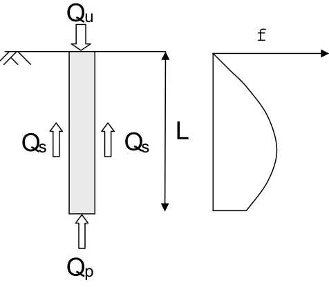
Prior to discussing the actual pile load tests performed and the results and conclusions from those tests, a brief review of pile capacity in general is provided. In general, as mentioned earlier, a pile in soil is effective as a deep-foundation solution because it most often transfers some axially-applied load to usually deeper soils and reduces settlement. This transfer of the load is a phenomenon that takes place due to the interaction of the soil and pile and the soil near the base of the pile. In other words, the ultimate axial capacity, Qu, that a pile can have is the summation of the skin friction developed between the sides of the pile and the soil, Qs, and the bearing capacity of the soil at the tip of the pile, Qp (Das, 2004) such that
s p
u Q Q
Q ………(Eq. 2.1)
This is shown in Figure 2.1 for a pile driven into a soil a distance, L, from the surface and summing axial forces.
Figure 2.1 Schematic showing a typical pile driven into soil and the forces
involved in determining pile capacity.
Once the pile is driven and sets up and the load that the pile must resist is increased, the load-carrying capacities along the shaft and at the tip are mobilized. The part of the load carried by the shaft varies along the length of the pile such that it is maximum near the ground surface and curvilinearly decreases down to the part of the load carried by the pile tip. Lymon Reese and his colleagues capture this generally-accepted explanation in Figure 2.2 (Reese et. al, 2006).
Q
sQ
Q
Q
s
p u
Figure 2.2 Schematic showing a typical pile driven into soil, the forces
involved in determining pile capacity, and the variation of the skin friction capacity with depth.
The unit frictional resistance along the shaft, f, on the other hand, is a ratio of the unit load-carrying capacity along the shaft, ΔQs, to the product of the perimeter of the pile, p, and the unit length along the shaft, ΔL, such that
L p
Q
f s
………..………..(Eq. 2.2)
This unit friction along the shaft varies such that it is zero near the ground surface, increases curvilinearly to some maximum value near 65% of the depth of the pile from the ground surface then curvilinearly decreases to some value greater than zero at the tip of the pile as shown in Figure 2.3.
Q
sQ
Q
Q
s
p u
L
Figure 2.3 Schematic showing a typical pile driven into soil, the forces
involved in determining pile capacity, and the variation of the unit friction resistance with depth.
The phenomenon of the axially-applied load being transferred to the soil and hence the load-carrying capacity of the pile is highly dependent on the method of installation (Reese et. al, 2006). Though piles can be installed via boring and vibrating, the piles that this research will focus on were installed via the common technique of driving. Other aspects that could affect the load-transfer process are the material the piles are being driven into and the types of piles
themselves. Next, the types of soils and the manner in which axial pile capacities are developed in each will be explained. Afterwards, the actual piles used at each pile load test site and their theoretical capacities will be discussed.
2.1.1 Piles in Clays
Because of the deltaic nature of the Mississippi River over time in southeastern Louisiana, the majority of the soils found are highly-stratified and composed of clays, sands, and silts that are relatively weak, especially the upper soils, when compared to soils across the nation.
Nevertheless, with the above general description of axial pile capacity in mind, the axial capacity in each of these soils is derived differently. To begin with, clay is a material that has cohesion among the particles that make it up. Clay particles are considered fine-grained (Coduto, 1999) and have relatively low permeabilities since the particles are closely spaced. Because of its cohesive nature, the skin friction part of the equation is based on the unit skin friction resistance, f, described above and the side surface area of pile. Though there are numerous methods to determine each of these parts, only the method that will be used to determine actual axial capacities will be discussed. The unit skin friction resistance, f, developed between the pile and the clay is a function of the undrained shear strength of the normally-consolidated clay, c, and the effective overburden on the stratum of clay, σ’o, in question. This method is referred to as the Revised API Method (1987) (Reese, 2006) and the equation is
f
Q
sQ
Q
Q
s
p u
5 . 0
5 . 0
if 1.0……….………(Eq. 2.3)
25 . 0
5 . 0
if 1.0………..…………...(Eq. 2.4)
where
'
o c
……….……….………..(Eq. 2.5)
Once the alpha coefficient is determined, it is combined with the cohesion value to produce the unit skin friction resistance value (Reese, 2006) such that
c
f ……….(Eq. 2.6)
This is then combined with the side surface area of the pile, As, which is simply the product of the perimeter of the pile, p, and the length of clay along the pile, L, to obtain the load-carrying capacity along the pile shaft such that
cpL fA
Qs s ………(Eq. 2.7)
If there are varying clay strata present that the pile in question is driven into, Equation 2.7 can be modified (Das, 2004) such that
L
s p c L
Q
0
……….………..(Eq. 2.8)
For cohesive materials, the bearing part of the axial-load-carrying capacity, Qp, is based on the cohesion of the soil that a pile would be tipped in and the end area of the pile. The API Method simply states the unit end-bearing resistance, q, to be 9 times the undrained shear strength (Das, 2004) or
c
q9 ………..………..(Eq. 2.9)
It is worth noting that for this method, the undrained shear strength is taken as the average over a distance of two pile diameters below the tip of the pile. Once the unit end-bearing is determined, one can determine the end-bearing for a particular pile if the cross-sectional area of the tip of the pile, Ap, is known such that
p
p qA
Q ……….………...(Eq. 2.10)
Depending on the type of pile in question, this cross-sectional area may require some
Figure 2.4 Typical H-pile and pipe pile that both have hollow segments in their
cross-sections.
Consequently, instead of displacing the soil as they are driven, these piles interact with the soil. Especially given the nature of the soils in southeastern Louisiana, there is a good possibility the hollow parts of the tips of these types of piles will be filled with what is referred to as a soil plug unless the contractor elects to weld a plate at the pile tip across the hollow section creating a displacement-like effect. Nonetheless, for the open-ended steel piles, the soil plug complicates the end-bearing calculation because the cross-section at the tip is now composed of steel and some form of a soil plug. This soil plug is often conservatively assumed to have remolded strength since it is disturbed. This is left to engineering judgment.
Figure 2.5 Cross-section of a typical H-pile and schematic showing
conservative method for determining unit skin friction for typical H-pile.
It is worth mentioning that in theory the weight of the soil plug itself can affect the ultimate load-carrying capacity of the steel pile. As the open-ended steel pile mechanically becomes a
displacement pile when the soil plug no longer moves up the shaft, the weight of the soil plug becomes added weight applied to the foundation soils. To account for this additional weight, the pile capacity (i.e. in tons) should be reduced by the weight of the soil plug (i.e. also in tons).
2.1.2 Piles in Sands
With the major two parts of the axial load-carrying capacity defined for piles in cohesive
material such as clay, it is fitting to compare this to that for piles in cohesionless material such as sands. The two parts are similar but the manner in which each is obtained is different for sands. To start with the frictional resistance can again be generally stated as
fA fpL
Qs s ………..…..(Eq. 2.11)
The perimeter, p, and the unit length, L, of a particular stratum of sand along the shaft of the driven pile is fairly straight-forward and is explained above. The unit friction, f, is more
complex. Unlike cohesive soils, as a pile is driven into sands and the vibrations from the driving hammer travel down the pile, researchers have field-verified that the soil immediately adjacent to the pile gets densified. This means that the effective internal angle of friction of the sand, φ’, increases by approximately 6-15% (Das, 2004). In general, the unit friction, f, starts from zero at the intersection of the ground surface and the driven pile, increases with depth slightly
curvilinearly to a critical depth 10-20 pile diameters from the ground surface depending on the relative density of the soil, then remains constant to the tip of the pile (Reese, 2006). This can be seen pictorially in Figure 2.6.
Soil to Soil
Steel to Soil
Figure 2.6 Schematic showing a typical pile driven into sand, the forces
involved in determining pile capacity, and the variation of the unit friction with depth.
The unit friction, f, is not only a function of the angle of friction between the cohesionless soil and the pile, δ, but also the effective overburden pressure at a particular stratum, σo’, and the lateral earth pressure coefficient, k, (Das, 2004) such that
' tan
o k
f ………(Eq. 2.12)
It is worth mentioning that the vertical effective stress will vary down to the critical depth and then will remain constant helping to produce the general variation shown in Figure 2.6. The values of the lateral earth pressure coefficient using the U.S. Army Corps of Engineers Method can be taken as 1.00-2.00 if the pile is in compression, kc, and 0.50-0.70 if the pile is in tension, kt (Reese, 2006). Also, the values of the adhesion between the cohesionless soil and the pile depend on the soil’s own internal angle of friction and the material of the pile driven
(Department of the Army, 1991) as stated in Table 2.1
Table 2.1 Adhesion values between cohesionless soils and piles
Pile Type Δ
Steel 0.67φ to 0.83φ
Concrete 0.90φ to 1.00φ
Timber 0.80φ to 1.00φ
The values for δ in Table 2.1 apply to piles that are driven rather than vibrated or jetted.
The second part of the load-carrying capacity of a pile driven into cohesionless soil such as sand is the end-bearing. Similar to that of a cohesive material, the end-bearing is again based on the
f
L
’
Q
sQ
Q
Q
s
p u
unit end-bearing resistance, q, of the cohesionless soil at the tip of the pile which is further a function of the angle of internal friction of the soil, φ, at the tip of the pile and a bearing capacity factor, Nq, that can be simply read from a chart similar to Figure 2.7 (Reese, 2006).
Figure 2.7 Angle of internal friction vs. bearing capacity factor for cohesionless
soils
Once the soil’s angle of internal friction is known and the bearing capacity factor is read from Figure 2.7, this factor is multiplied by the effective overburden at the pile’s tip to give the unit bearing capacity (Department of the Army, 1991) and this unit bearing capacity is then
multiplied by the area of the pile tip to give the end-bearing load-carrying capacity of that particular pile driven in that particular cohesionless soil such that
p q o p
p qA N A
With respect to the end area of a pile, a pile driven into a cohesionless soil is similar to a pile driven into a cohesive soil. The pile is not a true displacement pile. Once the engineer
conservatively determines the end area and Equation 2.13 is calculated, the total capacity of the pile driven into that cohesionless soil can be determined by combining Equations 2.11 and 2.13 such that
( ) ( ) ( ) ( ' ) [ ( ' tan ) ] ( ' ) p q o o
p q o p
s p
s
u Q Q fA qA fpL N A k pL N A
Q …...
………(Eq. 2.14)
2.1.3 Piles in Silts
Because southeastern Louisiana is alluvial, there is a good chance that a particular area in southeastern Louisiana will have some silt present. Therefore, the method for determining the axial load-carrying capacity of a pile driven into a silt material will be described. Silt material is unique in that it is similar to both cohesive and cohesionless soils. Silt has cohesion but
individual particles are larger than clay particles causing larger void spaces and less contact area between particles (Spector, 2001). Because of the voids and the orientation of these particles, silt will usually have less cohesion than clay. On the other hand, silt also has an internal angle of friction. Though silt particles are usually larger than clay particles, they are usually smaller and usually have smaller void spaces than sand-type particles. This results in silt having a smaller internal angle of friction than that of the sand. Therefore, since silt material has both cohesion and internal friction, if a pile is driven into this type of material, accepted practice is for the engineer to use both sets of equations described above for both friction along the shaft and end-bearing. Thus, the load-carrying capacity along the shaft in silt can be determined using the following equation (Department of the Army, 1991)
) tan
( '
c D
k pL
Qs ………..…………(Eq. 2.15)
where again k is the lateral earth pressure coefficient and γ’D is the product of the effective unit weight and the depth from the ground surface collectively referred to as the vertical effective stress as explained in Equation2.12. The axial load-carrying capacity near the tip of the pile bearing on the silt can be determined using the following equation (Department of the Army, 1991)
q o p
p A N
Q ' ……….………..(Eq. 2.16)
2.1.4 Piles in Stratified Soils
The above discussion is theoretical and quite practical for piles driven in homogenous clay, sand, or silt individually. However, as also stated several times above, the soil native to southeastern Louisiana is highly stratified, which means it is very common to find clay, sand, silt, and other minor classifications of soil in layers on top of one another varying in thicknesses. Determining the axial load-carrying capacity of a pile in this scenario is not any more complicated than of a pile driven into one of the homogenous materials, but it is a little more time-consuming because the engineer has to perform the appropriate set of calculations at each strata. Also the end-bearing capacity is determined from whatever strata the pile is tipped into.
The U.S. Army Corps of Engineers expands on these general concepts and applies conservatism to the determination of the axial load-carrying capacity via the following guidelines. End-bearing can be counted if the tip is in cohesive material if the cohesion is greater than 1000 psf. Effective overburden for a particular stratum is usually limited to 3500 psf. Finally, end-bearing can only be counted on if the pile is 8 pile diameters or five feet up from the bottom of that strata to avoid what is referred to as “punch through,” especially if the soil beneath the bearing strata is weaker in nature than the bearing strata. Computers make applying these guidelines and theory to a unit length along the pile shaft easy. The software Pile Capacity allows the user to input a particular pile’s properties and the foundation material the pile will be driven into. Based on the theories explained throughout Section 2.1 above and the specified pile and foundation material types, the software incrementally calculates the pile’s theoretical ultimate capacity and a pile curve is developed.
It is clear that the perimeter of the pile is a major part of the unit skin friction determination regardless if the soil is cohesive, cohesionless, or both. H-piles (i.e. HP 14x73) were historically the primary choice for the deep foundation for T-Walls, and an H-pile cross-section is typically analyzed with a steel-to-soil component and a soil-to-soil component as shown in Figure 2.5. An HP 14x73 has a flange width of 14.585 in. and a depth of 13.61 in. With the soil plugs
considered, the perimeter of the cross-section of an HP 14x73 can then be conservatively taken to be 56.39 in. USACE’s Spiral Welded Pipe Pile Innovation Team calculated that a spiral welded pipe pile with an outer diameter of 18 in. will result in a perimeter of 56.5 in., which is very close to that of the HP 14x73. Likewise, Table 2.2 provides perimeter information for types of piles associated with this research.
Table 2.2 Perimeters for typical piles
PILE TYPE
DIMENSIONAL NOTES
PERIMETER, in.
Hence, if the perimeters are the same, both are made of steel, and both are driven into the same foundation material, load-carrying capacities of the two should be the same. This theory and its results will be discussed later in the research. It is worth mentioning that the Spiral Welded Pipe Pile Innovation team tested other diameter spiral welded pipe piles in addition to the 18 in. o.d. under the same principles. The Innovation team also determined that the ratio of the outer diameter of a spiral welded pipe pile to the thickness of the walls of that spiral welded pipe pile should be less than or equal to a non-dimensional value of 55 (USACE-MVN2, 2010).
2.2 Lateral Capacity
Deep foundations are not only useful for transferring axial loads from a weaker stratum and reducing settlement, but they are also useful in resisting horizontal or lateral loads, such as earthquake forces or horizontal wave loads. From a structural engineering perspective, this type of load in essence creates a bending force in the pile that can be related to bending in a beam. In some instances, the axially-applied load discussed above can affect the lateral considerations such that the pile has to be treated as a beam-column, but this is only in special instances. The pile’s ability to safely resist this bending, or in other words the pile’s lateral capacity, is a function of the stiffness of the pile and the soil, the fixity of the ends of the pile, and the
interaction between the pile and the soil. Because of the variability of these factors with depth, a complex differential calculation has to be made to obtain the theoretical lateral capacity of the pile.
The overall governing form of the differential equation including effects from an axial load can be stated as follows (Reese, et. al, 2006):
0
2 2
4 4
E y
dx y d P dx
y d I
Ep p x py ………..…..(Eq. 2.17)
where Ep and Ip are the elastic modulus and moment of inertia of the pile, respectively, or combined is the lateral stiffness of the pile, x is the distance along the pile, y is the lateral deflection of the pile, Px is the axial load if applicable, and Epy is the lateral stiffness of the soil. The lateral stiffness of the pile will be discussed first. The governing differential equation stated in Equation 2.17 can be managed by first making simplifying assumptions. Reese, et. al. offer the following key assumptions to be implored when addressing lateral loads on piles and Equation 2.17 (Reese, et. al, 2006):
a) the pile has a uniform, homogenous, isotropic cross-section
b) the pile’s modulus of elasticity is the same in both compression and tension c) dynamic loading of the pile is not considered
d) axial loads do not affect the pile
e) shear and moment equal zero at the pile tip
With these assumptions in place, the engineer then has to determine boundary conditions for the top of the pile in order to solve the differential equation. The top of the pile is normally
reduced, especially for concrete piles, as bending moment along the pile’s shaft increases (Reese, et. al., 2006).
With that above assumptions and published equations, an engineer would be able to correlate a deflection of the top of the pile to the anticipated lateral load. He or she would also be able to calculate slope, moment, and shear along the length of the pile.
Professional geotechnical engineers have acknowledged and it is now standard accepted practice that in order for an engineer to get a complete feel for the behavior of a pile under lateral loading, the reaction of the soil adjacent to the pile with respect to the laterally-applied load needs to be calculated as well. The engineer can accomplish this by producing a family of “p-y” (or soil response-pile deflection) curves at different depths along the pile for varying loads. A typical p-y curve can be broken into several portions. The beginning portion of the curve is linear and nearly vertical and is sometimes considered to resemble the stress-strain relationship of the soil in question. The end portion of the curve is also linear but is nearly horizontal and can be taken to resemble the ultimate bearing capacity of the soil in question. This near horizontal portion indicates that as strain increases, the shear strength remains constant, or in other words, as the pile deflection increases, the soil response remains constant. The middle portion is curved and connects the beginning portion to the end portion in a calculated fashion. For the middle portion of the curve, the engineer again uses published equations to determine the deflection
corresponding to half of the ultimate soil resistance, the deflections corresponding to the ends of the middle portion of the curve, and then deflections corresponding to different soil resistances that would complete the middle portion of the curve. The shape of this middle portion signifies that the soil response increases at a decreasing rate as the deflection of the pile increases. The shape of the p-y curve overall can indicate to the engineer if the soil will remain in its elastic state or be deformed due to the applied loading. Typical p-y curves can be seen in Figure 2.8.
Figure 2.8 Typical p-y curves at different depths along a pile’s shaft
It is worth mentioning that if the lateral loads anticipated are considered “sustained” in nature and the soil adjacent to the pile is clay of soft to medium consistency, which again is very typical for the southeastern Louisiana region, the lateral load will actually increase the pore water
that soil will actually occur, even though consolidation is usually thought to occur in the vertical direction, and the deflection of the pile will increase (Reese, et. al., 2006). Also, if the loads are cyclical, the p-y curves will not be affected for small deflections, but for larger deflections, the soil will actually lose resistance.
It is also worth mentioning that modifications to the p-y curve should be made if the ground is sloping instead of horizontal, if the pile is battered instead of vertical, if the pile is founded in rock, if free water is present, and if a considerable axial load that affects the bending moment of the pile is present. However, these special considerations will not be addressed in this research.
With these guidelines, the pile stiffness and the p-y curves can be developed and the engineer can predict how the lateral load is resisted. Example lateral response calculations performed on an 18” outer-diameter spiral welded pipe pile from one of the pile load test sites described in Chapter 3 can be found in Appendix C. The above theories for determining pile capacity related to both axially-applied and laterally-applied loads are used to help predict the behavior of the piles that the remainder of this research will focus on.
2.3 Field Capacity of Piles
Theoretical behaviors of piles are quite useful when an engineer has to design a structural component using those piles. However, theory is worthless to society if it is not tested and thus proved or disproved and if the results are not documented for future reference. Piles can be statically or dynamically tested, and analyses associated with each can be performed. Below, static testing and analyses will be explained as well as dynamic testing and analyses.
2.3.1 Static Testing
Figure 2.10 Schematic showing a typical tension pile load test setup.
For all three pile load tests types, a hydraulic ram (i.e. jack) creates the required loading force for the test to proceed, while some sort of reaction system forces this load to the test pile.
For a typical compression pile load test, the ram is placed between the test pile and the reaction beam. As the ram extends, it pushes downward on the test pile essentially putting it into compression while pushing up on the reaction beam, which is connected to the reaction piles putting them essentially into tension. Similarly, for a typical tension pile load test, the reaction beam is placed between the test pile and the ram, and the ram is separately connected to the test pile by a plate and large threaded bolts. As the ram extends, it pushes downward on the reaction beam and hence on the reaction piles putting them into compression while pushing up on a plate connected to the test pile putting it in tension.
For a typical lateral pile load test, the ram is placed in a horizontal orientation adjacent to test pile. The “reaction system” can either be another test pile or reaction piles. For instance, the set-up in Figure 2.11 is for two test piles. If the set-set-up is two test piles, as the ram extends, it loads and tests both piles simultaneously. Otherwise, as in a compression or tension test, as the ram extends, the load is applied to the single test pile, while the reaction system’s behavior is noted for information only. This explanation of axial and lateral load testing is applicable to all pile load tests that were performed in conjunction with this research and that will be discussed below.
2.3.2 Static Analyses
Once the pile load test is performed in the field on a particular pile, the raw data is made available to the engineer. It is then up to the engineer to determine if the test pile has satisfactorily resisted the design service load, which is normally considered to be the worst axially load the pile will see multiplied by a factor of safety. There are numerous methods accepted and used by engineers to make this specific determination; however, all methods normally start by having the engineer plot the raw “load versus deflection” data, which is the result of the pile being loaded and unloaded to specific percentages of the service load and the top of the pile moving with respect to its original elevation depending on these specific loadings. The U.S. Army Corps of Engineers’ pile load test specifications (Sec 31 62 18.00 12) for
Table 2.3 USACE typical load-and-unload cycles for pile load tests
Load/Unload Cycle
% of Service Load
Load/Unload Cycle
% of Service Load
50% 0% 200% 0%
25% 50%
50% 100%
25% 150%
0% 175%
100% 0% 200%
50% 150%
75% 100%
100% 50%
75% 0%
50% 300-500% 0%
0% 50%
150% 0% 100%
50% 150%
100% 200%
125% 210%
150% 220%
125% 230%
100% …
50% n%
0% 75%n
50%n
25%n
0%
All the pile load tests associated with this research followed these exact specifications. An electronic form of this spreadsheet is very helpful in managing the readings and later making plots of this data.
Once the raw data is obtained by the engineer from the pile load test, the load and deflection values are plotted both on arithmetic scales. The applied load can then be increasingly plotted on the x-axis and the deflection can increasingly be plotted downward on the y-axis. If these
methods of plotting are adopted, the curve that normally results can be broken into distinct parts. The test results will normally have a positively-decreasing-sloped curve for the loading portion of the test up to a maximum. The test results will often have a near-vertical component
representing a change from loading to unloading and meaning that for the same load a relative amount of deflection occurs. Finally, the test results will normally have a rebound-type
negatively-increasing-sloped curve from the unloading. The path that this curve takes represents the elasticity of the pile itself (FHWA1, 2006). If the unloading curve doesn’t get back to the exact deflection value that loading portion started out with, the difference between the unloading and loading can be attributed to a rearrangement of Hooke’s Law in one dimension that states the stress is the resultant of a strain and the modulus of elasticity (Beer, et. al, 2001)
E
………...…..………..(Eq. 2.47)
such that the sustained deformation, δ, is
AE PL
……….……….(Eq. 2.48)
Figure 2.12 Schematic showing a typical load-and-unload cycle for a pile load
test
Once the original data is plotted in the above format for each of the loading cycles, there is no industry-accepted single method for evaluating the test pile’s load-carrying axial capacity. One such method is referred to as the Davisson Method and was developed by M.T. Davisson in the early 1970s (FHWA2, 2006). For this method, the engineer constructs a line starting at a point with zero load and approximate deflection of 0.3 inches. In some cases, the deflection point is calculated as
) 008 . 0 38 . 0
( D
AE PL
Sf ………..………(Eq. 2.49)
in the case that 100% of the load, P, is transferred to the toe and D being the diameter of the pile (FHWA2, 2006). Once this initial point is determined, a slope parallel to the
unloading/reloading cycle of the pile load test’s raw data is constructed. Where this sloped constructed line intersects the plotted raw data on the final-loading curve is considered to be the ultimate axial capacity of that pile (FHWA1, 2006). Though this method does take into account the properties of the pile and the load-transfer along the pile, it often overestimates the deflection or settlement of the top of the pile for load-settlement records based on holding the main design load for 24 hours or longer (Peck, et. al., 1974) and is not practical for load-and-unload cycle tests. Since all of the static pile load tests associated with this research follow this exact criteria of holding the main design load for 24 hours and going through the load-and-unload cycles, Davisson’s Method will not be used in the determination of the capacities for these piles.
A second method is referred to as the Hansen Method or the Hansen’s 80% Criteria Method. It was developed by J. Brinch Hansen in 1963 (Fellenius, 2001). In this method, for each load-deflection reading, the square root of each load-deflection is divided by its corresponding load and this quotient is plotted against deflection on the original load-deflection curve. The engineer can then best-fit a straight line through the plotted quotients and determine the slope of the straight line, C1, and this line’s intercept of the “load” axis, C2. Hansen’s interpreted ultimate capacity,
Load (tons)
0 50 100 150 200
Deflection (in.)
0 .0002 .0004 .0006 .0008 .001 .0012 .0014 .0016
Qu, for that test pile at an associated ultimate load, δu, can then be determined from the following relationships (Fellenius, 2001):
2 1
2 1
C C
Qu ……….………..(Eq. 2.50)
and
1 2
C C
u
………..……….(Eq. 2.51)
In some cases, the point (Qu, δu) incorrectly falls a distance from the raw-data curve and should be corrected if necessary.
A third method is referred to as the De Beer Method (Abdelrahman, et. al., 2003). It was developed by E.E. De Beer. In this method, each load-deflection point obtained during the pile load test is plotted on a log-log scale. Once these are plotted, an engineer best fits a straight line through the top group of readings and a second through the bottom group of readings, since there theoretically should be an obvious break in the plotted data (Abdelrahman, et. al., 2003). The intersection of these two straight lines is considered the pile’s “yield” load, which is considered to mean something different than the ultimate load which all of the other methods use.
A fourth method is referred to as the Chin-Konder or Modified Chin Method (Sands, 1992). It was developed by Chin Fung Kee in 1970 and presented at the Second Structural Engineering Conference of Soil Engineers. With this method, the engineer calculates the ratio of deflection or settlement to load for every load-deflection reading of the pile load test and plots this ratio value on one axis against the associated deflection or settlement value on the other axis and best fits a straight line through these plotted values. The engineer then calculates the inverse slope of this best-fit line which gives the ultimate capacity for that test pile (Sands, 1992).
A fifth method of interpreting the data is the Mazurkiewicz Method. This method was developed by B.K. Mazurkiewicz in 1972 (Abdelrahman, et. al., 2003). For this method, equal intervals of pile deflection or settlement are selected on the load-deflection curve and loads corresponding to these deflections are marked on the load axis. From each mark on the load axis, a line with a 45° angle counterclockwise from horizontal is drawn to intersect the next marked load value until all marked load values are intersected. The engineer then constructs a best fit line through these intersection points of the 45° line and the next vertical marked load line, and where this best-fit line crosses the axis is considered the ultimate capacity for that test pile (Abdelrahman, et. al., 2003).
Similarly, the “gross” values of the same final load for each cycle are then connected by a separate best-fit curve. To better explain the difference between net and gross values, Table 2.6 provides a set of load and deflection points from a hypothetical cycle of loading and unloading.
Table 2.5 Example load and unload cycle for a pile load test
% of Service Load
Elapsed Time, min
Deflection, in
0% 0 0
25% 2 0.0135
8 0.014
15 0.0155
30 0.0185
60 0.0225
120 0.029
50% 2 0.042
8 0.0435
15 0.0425
30 0.0455
60 0.048
120 0.0585
25% 20 0.0255
0% 20 0.0135
From this hypothetical 50% load/unload cycle, this pile was subjected to 25% of the design service load and readings were recorded at specific increments of time. The pile was then subjected to 50% of the design service load and readings were again recorded at specific increments of time. The pile was then unloaded back down to 25% and ultimately 0% of the design service load and readings were again recorded at specific increments of time. Since this is a 50% load/unload cycle, the deflection at the last reading of the 50% loading, in this case a value of 0.0585 in., would be plotted for the “gross” curve. Also, for any load/unload cycle, once the pile is loaded and then unloaded, the deflection once the load is completely removed is considered the net value of the curve. Thus, for this hypothetical example, a value of 0.0135 in. would be plotted for the “net” curve. Likewise, the gross and net points associated with all the load/unload cycles for the test pile are determined and gross and net curves are formed.
With these two curves plotted, the first technique under the Corps of Engineers Method is referred to as the “gross curve” technique. Here, a line with a 0.01 in/ton creep rate is
again considered the ultimate capacity of that test pile for this technique (Department of the Army, 1991).
Once the three techniques are performed and the corresponding three ultimate capacities are determined, the engineer then decides if all three should be used. The techniques that are used are normally averaged together resulting in a final ultimate load-carrying capacity of the test pile. Though the first five methods mentioned will not be directly used to reduce each pile load test associated with this research, several of these methods were performed on one selected pile load test and the results are presented for comparative purposes in Table 2.6.
Table 2.6 Comparison of several reduction methods on a selected pile load test
METHOD
ULTIMATE CAPACITY
USACE 127 Tons
Gross Curve (Creep) 121 Tons
Tangent 132 Tons
0.25 Inch 127 Tons
DAVISSON 132 Tons
HANSEN 94 Tons
Six methods were discussed above, but it is worth mentioning that there are numerous other methods used world-wide to interpret pile load test results and determine a pile’s ultimate capacity that will not be listed here. An engineer may also be concerned with dynamic analyses as explained below.
2.3.3 Dynamic Testing
Besides the two types of static pile load tests described above, another type of test that can be performed on the pile to obtain capacity is considered a dynamic test. Dynamic testing can actually be broken into two types, initial testing and restrike testing. For both types, standard procedures call for calibrated transducers and accelerometers (i.e. at least two of each if the USACE specifications are followed) to be securely attached to the pile near the top of the pile.
For the initial testing, once the transducers and accelerometers are attached to the pile, the contractor applies impacts or blows via an impact driving hammer axially and concentrically to the pile. As the impacts are applied, the contractor in charge of the dynamic testing records number of blows, the driving stresses, the force and acceleration signals at the top of the pile, the integrity of the pile and driving system, performance of the cushion and hammer, and the soil’s resistance to those blows.
for 21 days before the restrike dynamic test can be performed (USACE Guide Specification, Section 02355-23). After the set up is allowed to occur, the contractor shall warm the impact driving hammer up then apply 50 blows to the pile or until the pile is driven an additional three inches into the ground.
2.3.4 Dynamic Analyses
Any dynamic test associated with this research and most that USACE are associated with follow ASTM D4945 (2008). Before a test pile or production pile is ever driven, a critical piece of information needed for dynamic testing comes from the development of a wave equation specific to the pile type being tested. This wave equation is a one-dimensional differential equation that takes the following form (Warrington, 1999):
) , ( )
,
(x t E u x t
utt xx
……….……….………(Eq. 2.52)
where u(x,t) is the displacement of pile particle in meters, x is the distance from the top of the pile in meters, t is the amount of time in seconds, E is Young’s Modulus of Elasticity of the pile in Pascals, and ρ is the density of the pile in kg/m3. This equation is transformed by introducing boundary conditions of the specific system, especially whether it is a dampened or undampened case. For the case where dampening along the pile shaft is not present, the critical equation becomes (Warrington, 1999)
1 21 cos 1 sin 1 ,
cos ) , ( n n n n n n c L t L tc C L tc C L x t x
u
………..………..…..…….(Eq. 2.53)
and for the case where there is dampening along the pile shaft, the critical equation becomes (Warrington, 1999)
( )( )
( ) , 01 ) , ( 0 2
2
t o o b t d t F a b I e Z t x
u ……..…..…(Eq. 2.54)
where λn is the Constant of Eigenvalue, L is the length of the pile in meters, C1n and C2n are Constants of Fourier Coefficients, c is the acoustic speed of pile material in m/sec, Z is the pile impedance in N-s/m, b is the pile shaft dampening constant in 1/sec, τ is a dummy variable, a is the pile shaft elasticity constant in 1/sec2, and Fo is the force at the top of the pile in Newtons.