VOLUME 38, ARTICLE 50, PAGES 1535
,
1576
PUBLISHED 3 MAY 2018
http://www.demographic-research.org/Volumes/Vol38/50/ DOI: 10.4054/DemRes.2018.38.50
Research Article
A regional perspective on the economic
determinants of urban transition in
19
th-century France
Philippe Bocquier
Sandra Brée
© 2018 Philippe Bocquier & Sandra Brée.
This open-access work is published under the terms of the Creative Commons Attribution 3.0 Germany (CC BY 3.0 DE), which permits use, reproduction, and distribution in any medium, provided the original author(s) and source are given credit.
1 Introduction 1536
2 Methods and data: timing of urban and vital transitions 1539
3 Results 1544
3.1 The contribution of migration, reclassification, and natural
movement to urbanisation at the national level (1821–1891) 1545 3.2 The contribution of migration and natural movement to
urbanisation for different types of economic development (1856–
1891) 1551
4 Discussion 1559
References 1562
A regional perspective on the economic determinants of urban
transition in 19
th-century France
Philippe Bocquier1
Sandra Brée2
Abstract
BACKGROUND
Past analyses lead to contradictory results as to whether migration, demographic transition, or economic development is the main driver of urban transition. Results depend heavily on the analytical strategy.
OBJECTIVE
This paper’s aim is to identify different profiles of economic activity and their effect on urban transition over the 19th century in France to test three hypotheses: economic
development acts on urban transition through migration; political and economic shocks better explain variations in the migration component of urbanisation than its natural components; the diffusion of the urban growth model of large cities explains urban transition in peripheral areas.
METHOD
The paper uses census data from 80 French counties – excluding Paris, Corsica, and counties disputed by Germany and Italy – for 1856 to 1891. Each component of urbanisation at county level is regressed on employment structure, controlling for neighbouring urbanisation and for distance to Paris and nearest large city.
RESULTS
Results confirm conclusions for Sweden and Belgium demonstrating that migration drove 19th-century urban transition. The migration component of urban transition is far more sensitive to employment structure and to political and economic instability than the natural components. The diffusion effect is marginal.
1 Centre de recherches en démographie, Université catholique de Louvain, Belgium.
Email:[email protected].
2 Centre National de la Recherche Scientifique, Laboratoire de Recherche Historique Rhône-Alpes, France.
CONCLUSIONS
Results concur with the hypothesis that the redistribution of economic production through migration, and not the demographic transition, drove the urban transition.
CONTRIBUTION
The relationship between economic development and urban transition is assessed through the interaction of employment profile and period. Similar methodology could be used to analyse urban transition in contemporary low- and middle-income countries.
1. Introduction
Demographers and economists have recently revived the debate on the drivers of urban transition – i.e., the change from a mainly rural to a mainly urban society – that was initiated by Zelinsky (1971). Like Bairoch (1988), who observed that the positive interaction between urbanisation and economic development in industrialised countries did not apply to developing countries, Fox (2012) points out that the presence of innovation in agriculture, transportation, and health may stimulate urban growth without economic growth, as observed in sub-Saharan Africa. Fox concurs with Dyson (2011) – who himself followed de Vries (1984, 1990) – who states that population growth through declining mortality may be a stronger contributor to urban transition than economic growth. Other authors consider that besides the better survival prospects in urban areas, it is mainly changes in economic production that increases net migration to urban areas, through land pressure, productivity increase, institutional changes, and other factors (Bocquier and Costa 2015).
The debate is not closed, since results seem to strongly depend on the countries, data, and indicators selected. In the field of demographics, Bocquier and Costa (2015) show that taking migration and reclassification3 components into consideration may lead to different conclusions than using birth and death data only, as Dyson (2011) did for Sweden. Trends in both Sweden and Belgium suggest that vital transition, i.e., the interplay of fertility and mortality, plays a secondary, unstable, and negative role in urban transition, while migration explains most of it in the long term. These conclusions for European countries call into question de Vries’s argument (1984) that spatially differentiated vital transition leads to urban transition, and reinstate Zelinsky’s hypothesis (1971) that mobility transition, and therefore the redistribution of economic
3 Reclassification may go both ways: rural (or urban) municipalities may be reclassified as urban (or rural)
production, drove the urban transition and not the demographic transition. Regarding the urban transition post-World War II, census data has shown that the contribution of natural growth to urban growth varied between 51% and 69% in 76 developing countries, depending on the period and the region (United Nations 2015). However, these figures do not reveal the extent to which natural and migration components of growth contribute to urban–rural growth difference, and consequently to the increase in the rate of urbanisation. Estimating the components of the contemporary urban transition remains a contentious issue, since the data to do so is unavailable or not readily accessible, even at country level.
In the economics field, several authors use econometric panel regression models to analyse the role of urban natural increase, GDP per capita growth, education, and other factors in contemporary urbanisation (Christiaensen, Gindelsky, and Jedwab 2013; Fox 2012; Henderson, Roberts, and Storeygard 2013). Baudin and Stelter (2016) use the generalised method of moments to build an urban and rural growth model that includes rural exodus as well as mortality and fertility components, using historical Danish data. They conclude that rural exodus was key to urban and economic transitions and that declining mortality played a positive yet marginal role in these transitions, which contradicts the conclusions on contemporary transitions made by the previously cited economists and Adams (2017) on long-term transition in England.
Our contention is that the larger the geographical scale, the more important and complex the hierarchical dependence between sub-spaces, be they states or lower administrative boundaries within states. By hierarchical dependence we mean that a space (a state at the international level or counties at the sub-national level) depends on another with greater economic and political power. It is important to consider interspace competition and centre–periphery hierarchy in any analysis of transition in a productive and reproductive (economic and demographic) system. In this regard, migration to urban areas within a sub-space or migration to other sub-spaces can be considered as a reallocation of human resources to the centres of economic power.
The relative importance of each component of the urban transition will depend on when, where, and how economic and institutional changes occurred, which makes each analysis very space- and time-specific and may prevent generalisation. The geographical level and the period in which these components are measured are important in order to account explicitly for local change in the relevant economic hierarchy. To control for hierarchical dependency it is important to explicitly model political and economic shocks in addition to structural political relations and economic dependence.
the same methodology to French provincial counties over the 19th century (1821–1891),
when the urban transition started in France. However, our purpose is slightly different: not only do we aim to identify the migration and natural components of urban growth but we link these components to the economic profile of counties. France has an advantage over other large Western European countries such as Germany and the United Kingdom in that municipality (commune) and county boundaries were consistent over the 19th century (with the exception of disputed counties; see next
section) and thus consistent series of population counts, births, deaths, reclassification, and occupation can be extracted from remarkably well-maintained statistical books. France is a sufficiently large country to be able to identify different economic activity profiles and their effect on urbanisation, although in our case the analysis will be limited to 1856–1891 due to data constraints. Our first hypothesis is that economic activity is driving the urbanisation process through its migration component and not through natural components, thus testing Zelinsky’s hypothesis against de Vries’. The coincident advantage of considering the second half of the century is that France went to war with the Prussian empire in 1870, which resulted in a major economic crisis in the 1870s. This political and economic shock represents a sensitivity test of the migration, natural, and reclassification components of urbanisation. By controlling for the interactions between each of these components and observation periods, we will explicitly model the effect of shocks on the urban transition. Our second hypothesis is that the 1870s shock explains much more of the variation in the migration component than the natural and reclassification components of urbanisation. This hypothesis tests the sensitivity of the urban transition to political and economic shocks through the variation in the migration component. Finally, our third hypothesis is that proximity to the highly urbanised Seine county (Paris) and to major cities (Lyon, Marseille, Bordeaux, Rouen, Nantes, etc.) impacts positively on urbanisation: the urban way of life would diffuse from the centre (Paris) to the periphery (possibly through major cities) and affect the components of urbanisation; e.g., by reducing mortality and fertility in the county’s urban areas or by increasing long-term migration flows to major cities rather than to nearer regional centres. Indeed, the city is a place of innovation and diffusion of techniques and demographic behaviours. It promotes the monetisation of the economy, facilitates social mobility and the matching of supply and demand of skilled labour, and extends industrial and agricultural production outlets (Bairoch 1996).
2. Methods and data: timing of urban and vital transitions
The following is a summary of the methodology used in Bocquier and Costa (2015) for Belgium and Sweden, complemented by some details from the French data. The idea is to use basic aggregated data on population, births, and deaths by area of residence to deduce the migration component of population growth without direct measurement of migrations. Rates of increase in time intervalh in ruralr and urbanu areas are defined as:
= − + + (1a)
= − + + (1b)
where the rates , , , are respectively the crude birth rate, crude death rate, net internal migration rate, and net international migration rate, all in periodh. In addition to the natural and migration components, urban reclassification growth ( , when, most of the time, a locality becomes urban just by crossing a relative or absolute population threshold or as decided by central authorities) and rural reclassification growth ( , when, more rarely, a locality becomes rural) should be accounted for in equations (1a) and (1b) whenever data permits. Reclassification may itself occur as a result of cumulated growth over the years through migration, natural growth, or a combination of both.
For the proportion of the population living in urban areas to increase, the difference between urban and rural growth is more relevant than the urban growth. Although population growth in both urban and rural areas usually owes more to natural growth than to migration growth, the urban–rural growth difference may originate in either higher urban–rural natural growth difference or higher urban–rural migration growth difference. Therefore, we are interested in all the components, including reclassification, of the urban–rural difference in population growth:
− = ( − ) − ( − ) + ( − ) + ( − ) + ( − ) (2)
To make the figures below easier to read, each difference in urban–rural rates in (2) is abbreviated:
∆G = ∆CBR – ∆CDR + ∆intM + ∆extM + ∆R (3)
rural difference in internal net migration, ∆extM for urban–rural difference in international net migration, and ∆R for urban–rural difference in net reclassification. It is enough to know the urban–rural growth difference (∆G) and the urban–rural difference in natural growth (∆N=∆CBR-∆CDR) to deduce the remaining components (∆intM+∆extM+∆R). Data on reclassification (∆R) is fairly easily collected using lists of localities by size. When data on births and deaths is also available for the reclassified localities, the migration (∆RM) and natural (∆RN) contributions to the reclassification component are computed such that:
∆intM + ∆extM = ∆G – (∆CBR – ∆CDR) – (∆RN + ∆RM) (4)
The total direct and indirect (i.e., through reclassification) contribution of migration to urban–rural growth difference is therefore:
∆intM + ∆extM + ∆RM = ∆G – (∆CBR – ∆CDR) – ∆RN (5)
∆Mtotal = ∆G – ∆Ntotal (6)
where:
total migration contribution = ∆Mtotal = ∆intM + ∆extM + ∆RM (7) total natural contribution = ∆Ntotal = (∆CBR – ∆CDR) – ∆RN (8)
All growth rates and growth differences will be given per 1,000.
French statistical Mouvements de la population yearbooks that include birth and death counts by county were published regularly from the 1800s, as well as censuses that were conducted every five years, with some exceptions (1826 and 1841 are not available and the 1871 census was postponed to 1872). Most of this historical data is available online through EHESS’s Centre for Historical Research website (https://acrh.revues.org/2890). Births and deaths in urban areas for the years 1821– 1824, 1876, 1887, and 1889 are missing. Therefore, the corresponding period’s total figures were extrapolated from figures for documented years. Certain other events and behaviours can bias birth and death counts. Indeed, according to Garden and Le Bras (1988), it is likely that 200,000 urban deaths due to the 1870–1871 Franco-Prussian war were unrecorded, half of which were outside the Seine county. Additionally, the practice that persisted in the 19th century of fostering children – with urban middle-class
fostered infants means that urban mortality rates and the urban–rural mortality difference were underestimated.
Our definition of urban areas differs from that used in the official statistical yearbooks, which considered all municipalities of more than 2,000 inhabitants as urban. The threshold of 2,000 for municipalities is often considered too low as a definition of urban areas, as it is more sensitive to population growth leading to reclassification of municipalities from rural to urban. For the 20th century a threshold of 10,000 is quite
common, but in the 19th century a threshold of 5,000 was more often used. This was
also the threshold used in Belgian statistical books during the same period.
We collected data on urban municipalities that are chefs-lieux (administrative centres) and cities of more than 10,000 inhabitants and removed thechefs-lieux of fewer than 5,000 inhabitants. The limitation of our data is that it does not capture cities of 5,000 to 10,000 inhabitants that are notchefs-lieux, since they are not identified in the original yearbooks. We were able to count the number of deaths and births for all
chefs-lieux that were reclassified (crossing the 5,000 threshold either way) and for all
municipalities that were reclassified as cities by reaching the threshold of 10,000. This enabled us to compute the contribution of migration and natural movement to reclassification. Given that employment data was consistent from the 1856 to the 1886 census, we had to limit our study of the impact of economic profile to the 1856–1891 period and to alldépartements except for the Seine (the county that includes the capital city, Paris), Corsica (because of its insularity), and those disputed by Germany and Italy over the 19th century, i.e., the regions of Alsace and Lorraine and the counties of Savoie
and Haute-Savoie. The Seine was excluded since it was already more than 80% urban at the beginning of the 19th century (Brée 2015). For convenience, we will use the term
‘provincial France’ for the 80 selected counties in our analysis.
neighbouring counties by computing the percentage that was urban in the total population of adjacent counties. Distance to closest large city and neighbouring urbanisation varies from one period to the next for each county depending on the development of the largest cities and on urbanisation in neighbouring counties. The three variables (distance to the capital city, distance to the closest large provincial city, neighbouring urbanisation) control for an external ‘diffusion’ effect of the urban growth model that might not be directly related to the ‘endogenous’ economic effect of the county’s economic structure. Finally, we also controlled for the non-linear pattern in urban–rural growth difference in relation to the urban proportion (Bocquier 2005, 2015) by including the urban proportion and its squared term as covariates, both varying from one period to the next.
Two variables reflect push and pull factors that could play a role in urban transition independently of employment structure, urbanisation level, and distance to main cities. The push factor is the county’s rural population density measure as the population of rural municipalities of fewer than 2,000 inhabitants (which includes most rural municipalities, i.e., excluding towns and cities) divided by the total number of hectares in the county. This rural density indicator is expressed in population per 1,000 hectares. This indicator does not perfectly capture land pressure since actual arable land area is not available, only the total area of the county. The pull factor is the availability of education, measured by the number of schools for all the county’s municipalities. Since data on schools was not always available at the time of the census, the indicator was first computed for the available years and then interpolated to the census years, no more than two years apart from the recorded years. This indicator is expressed as the number of schools per 10 municipalities.
The main independent variable is the employment structure for males. Unfortunately, female employment during the 19th century was often categorised as that
of the male spouse, ‘housewife,’ or ‘without occupation’ (Motte and Pelissier 1992; Schweitzer 2002). Analysis of civil registers has shown that the more humble the husband’s social category, the more likely it is that the woman’s activity will be known (Motte and Pelissier 1992). The employment of women in industry is better known because they had a profession distinct from that of their husbands. However, the data was not consistently collected over the study period and across sectors.
A Ward’s linkage cluster analysis was performed to classify counties according to the percentage distribution of the seven categories of employment. However, the clergy employment category is non-discriminant in the cluster analysis, and so the four classes are essentially the result of the six other employment categories. It is noted that the cluster analysis was performed on county–period unit of analysis; that is, each unit was the combination of a period and a county. That way each county can change cluster from one period to the next, depending on change in its employment structure. Four classes were easily identified (see dendrogram in Figure A-1), ranked, and labelled (approximate proportions of employment are shown in parentheses: see Table A-1 for exact figures). The resulting four classes are ordered here from most to least agricultural, the most industrialised with higher-than-average tertiary employment. These four classes clearly represent a hierarchy of income and productivity, since industrial and tertiary activities were generating more income than agriculture in the 19th century (Dormois 2005; Lévy-Leboyer and Bourguignon 1985; Marchand and
Thélot 1997):
1. Large majority (3/4) agriculture: other categories are lower than average. 2. Majority agriculture (2/3), below-average industry (1/5): this is the largest
category and closest to the average French provincial county over the study period except for 1881, when it was outnumbered by the third category. 3. Mostly agriculture (1/2), average industry (1/4), and higher-than-average
commerce/transport and ‘others’.
4. Much-lower-than-average agriculture (1/4), large industry (4/10), and higher-than-average commerce/transport and ‘others’.
the components of urbanisation, net of other effects (level of urbanisation and diffusion effects).
The seemingly unrelated regressions (SUR) model used for analysis belongs to the class of generalised structural equation models (GSEM). With this type of model, a set of equations is defined for different outcomes, but the error terms are assumed to be correlated, as they should be when outcomes for the same statistical units are actually related. The urban–rural growth differences in mortality, fertility, reclassification, and migration for the 80 provincial counties are regressed in four separate ‘seemingly unrelated’ equations on the employment cluster to which the county belongs, interacted with period, the urban proportion and squared term (to account for the potential non-linear effect of urbanisation), the urban proportion in neighbouring counties, and the distance to Paris and closest large city, also interacted with period. Because the four components of urban–rural growth difference could be correlated to each other, a GSEM accounting for covariance between each pair of the four components is preferred over four ‘completely unrelated’ regression models, one for each component. A robust estimation method was tested to avoid the possible influence of outliers, but no difference with the ordinary estimation method was found, which is reassuring as far as the quality of the data is concerned.
In addition to the regression results, we computed the percentage contribution of each component of urban–rural growth difference net of other effects (also termed the mean ‘marginal effects’ of the main independent variable, computed at the mean value of control variables) in each cluster. This is a way to compare the regression results directly to the descriptive results, and thus to assess the role of control variables and outliers. If the results do not differ, the descriptive variations are then largely due to the combination of cluster and period effects and marginally due to control variables. If they do differ from the descriptive results, then the combined cluster–period effects obtained from the regression model will be interpreted as the underlying effect of the employment structure on each component of urban growth over time, all things being equal.
3. Results
3.1 The contribution of migration, reclassification, and natural movement to urbanisation at the national level (1821–1891)
The population of France was 31.39 million in 1821 and reached about 38.34 million in 1891. As in most Western European countries, the urban transition really started in the 19th century. The percentage urban in provincial France (as defined by us; see above)
rose from 10.6% (3.04 million urban) in 1821 to 16.8% in 1856 (5.42 million urban), and 22.0% in 1886 (7.43 million urban). This is 10 to 15 percentage points less than the official definition that includes municipalities of 2,000 to 5,000 inhabitants and the Seine county, which increased from 83% to 94% urban in the same period using our definition against 94% to 99% with the 2,000 inhabitants threshold (Brée 2015). Using our definition of urban, the trend is similar with and without Seine county (Figure 1).
Figure 1: Proportion of urban population in France and provincial France
(1821–1886)
Note: Definition of urban:chefs-lieux of 5,000 inhabitants or more and other urban municipalities of 10,000 inhabitants or more.
Crude birth and death rates per 1,000 (Figure 2) show a downward trend over the 1821–1891 period, interrupted by a peak of mortality in the war period (1866–1872).
0
10
20
30
1821 1831 1836 1846 1851 1856 1861 1866 1872 1881 1886
Crude death rates are constantly higher in urban areas, thus confirming the ‘urban penalty’, although a sharp decrease in the urban crude death rate was observed in the 1836–1846 period. Crude birth rates were higher in urban areas prior to 1836 but did not differ much in urban and rural areas thereafter, being slightly lower in urban areas from 1836 to 1872. The downward trend in fertility for provincial France exemplifies here the singularity of French fertility in the European landscape. Even without considering the highly urbanised, low-fertility Seine county (Brée 2017), fertility had already started to decline in both urban and rural areas before the 19th century. Using
data from Henry’s survey, Bardet (1998) dates the first fertility decline at around 1790– 1800, whereas Knodel and Van de Walle (1979) suggest 1827 as the first year of decline, using Coale and Treadway’s definition (irreversible fertility decline of 10% or more compared to the pre-transitional value). The cities’ precedence in fertility decline (Sharlin 1986) has been observed several times, e.g., in Rouen and in Paris (Bardet 1983; Brée 2017; Bardet 1998).
Figure 2: Crude birth and death rates (per 1,000) in urban and rural
provincial France (1821–1891)
Overall, the natural growth rate (= CBR – CDR) is always positive in rural areas, even during the war period, while in urban areas it hovers around zero or is even markedly negative during the war period. These trends in provincial France thus
20
25
30
35
1821 1831 1836 1846 1851 1856 1861 1866 1872 1881 1886 1891
confirm the phenomenon of the ‘urban demographic sink’ (a prolonged negative natural growth) observed elsewhere in 19th-century Europe, despite the downward mortality
and fertility trends.
Despite the urban demographic sink attributed to natural growth, the total growth rate per 1,000 as shown in Figure 3 is always positive over the 1821–1891 period in urban areas, with many ups and downs of around +12.3 per 1,000 on average, while the total growth rate in rural areas (+0.3 per 1,000 over the whole period) shows a downward trend from positive in 1821–1851 (+3.6 per 1,000) to generally negative or nil thereafter (−1.6 per 1,000). This contrasts with the urban demographic sink previously identified in Figure 2. The difference can only be due to migration and to a lesser extent reclassification, as shown in the following analysis of the components of urban–rural growth differences.
Figure 3: Total growth rates (per 1,000) in urban and rural provincial France
(1821–1891)
Figure 4 depicts the difference in vital transition between urban and rural areas (∆CBR, ∆CDR, and the resulting ∆N) as well as the trends in urban–rural migration plus reclassification growth difference (∆RMG=∆intM+∆extM+∆R). In the 1821–1836 period, urban areas have higher crude birth and death rates than rural areas, leading to a typical case of ‘urban penalty’ (excess urban mortality) not quite compensated for by
-1
0
0
10
20
30
1821 1831 1836 1846 1851 1856 1861 1866 1872 1881 1886 1891
higher fertility. After 1836, urban areas experience lower crude birth rates than rural areas, but also higher crude death rates. Natural growth difference is thus detrimental to urban areas (∆N hovers around −4.2 per 1,000), at times because of mortality and at others because of fertility. The urban demographic sink is persistent and almost constant. This is different from both Sweden (excess urban mortality with not much urban–rural difference in births) and Belgium (births compensating for excess mortality in urban areas) (see Figures A-2 and A-3 in the Appendix).
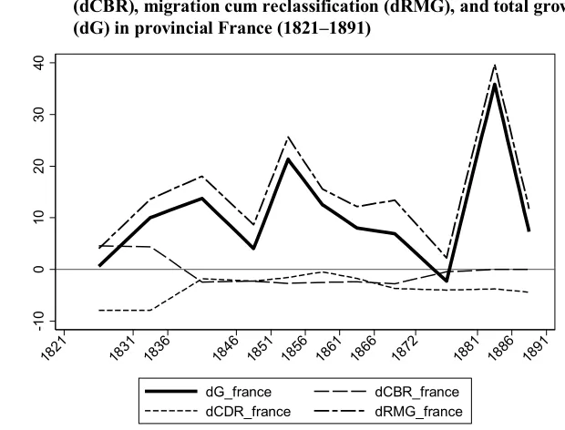
Figure 4: Urban–rural difference (per 1,000) in mortality (dCDR), fertility
(dCBR), migration cum reclassification (dRMG), and total growth (dG) in provincial France (1821–1891)
The most important trend depicted in Figure 4 is that migration together with reclassification highly contributed (correlation: 99.6%) to the level of and variation in urban–rural total growth difference (∆G), contrary to the natural component (correlation: 18.5%). Urban growth was mostly positive over the study period, with the noticeable exception of the post-war crisis period (1872–1881). This was the period following the turmoil of the Franco-Prussian war (1870–1871), various civil insurrections in several cities (the most famous in Paris in 1871), the fall of the Second Empire (Napoleon III), and the establishment of the Third Republic. Migration and reclassification bounced back in the 1881–1886 period. This period is characterised by
-1
0
0
10
20
30
40
1821 1831 1836 1846 1851 1856 1861 1866 1872 1881 1886 1891
the return of relative political stability and by economic recovery under the presidency of Jules Grévy, despite historians dubbing the 30-year period from the 1870 war to the end of the 19th century “the Long Depression” (Lhomme 1970).
Figure 5 repeats the total growth difference (∆G) and natural growth difference (∆NG) from Figure 4 but separates the migration component from the reclassification component. Total urban–rural growth difference per 1,000 is highly correlated with both reclassification (61.3%) and migration (91.9%), as compared to natural growth (only 18.5% correlation). Figure 5 shows that over the 1821–1891 period, reclassification made a positive contribution (+3.1 per 1,000 on average) while the migration contribution is nearly four times higher (+11.9 per 1,000 over the same period) despite being negative in 1872–1881. The 1881–1886 period shows a peak in urban–rural growth difference with a high contribution of migration and reclassification.
Figure 5: Urban–rural difference (per 1,000) in direct natural movement
(dNG), direct migration (dMG), reclassification (dR), and total growth (dG) in provincial France (1821–1891)
As explained in the methods section, we were able to further separate the natural and migration components of reclassification. Actually, 99.75% of reclassification (+3.1 per 1,000 on average over the study period) is explained by migration and the rest
-1
0
0
1
0
2
0
30
40
1821 1831 1836 1846 1851 1856 1861 1866 1872 1881 1886 1891
by natural movement. Therefore, the indirect contribution (through reclassification) of natural movement adds very little to the direct negative contribution (−4.2 per 1000) of natural movement to overall urban–rural growth difference.
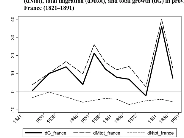
Drawing the indirect and direct contributions as two separate trends for natural and migration growth (Figure 6) shows quite clearly that in provincial France the overall level and variation of the urban–rural growth difference is determined by migration. The correlation of natural movement with urban–rural growth difference over the whole study period is very weak (12.8%) compared to the migration component (98.5%). The data shows that migration was the main and positive contributor to the French urban transition in the 19th century, while natural movement contributed negatively but
marginally to hampering it.
Figure 6: Urban–rural difference (per 1,000) in total natural movement
(dNtot), total migration (dMtot), and total growth (dG) in provincial France (1821–1891)
Trends in France as depicted in Figure 5 are interesting to compare with those of Belgium (Figure A-2) and Sweden (Figure A-3). The characteristics of the urban demographic sink are not universal. In Sweden this sink, observed prior to 1850, was essentially due to excess mortality in urban areas, and was gradually eliminated in 1850–1880. In Belgium there is no evidence of the urban demographic sink prior to the
-1
0
0
10
20
30
40
1821 1831 1836 1846 1851 1856 1861 1866 1872 1881 1886 1891
urban transition: a slight urban excess mortality was compensated for by excess fertility in urban areas up to 1900. If there was a sink it was rather weak and occurred after urban transition started and was mainly due to a birth deficit in urban areas in the first half of the 20th century. In provincial France there was a prolonged urban demographic
sink due to higher urban death rates and often-lower urban birth rates.
In Belgium over the 19th century, reclassification contributed more than twice as
much to the urban–rural growth difference than the migration component, and about half of this reclassification was due to migration. In Sweden the contribution of reclassification is positive but low before World War I. In France, reclassification contributed much less than the migration component and was largely due to migration, thus adding to its direct effect.
Replicating the analysis on historical demographic series for France has confirmed the conclusion drawn from Belgium and Sweden. At the national level of the three countries, the direct and indirect (through reclassification) role of migration was prominent in the urban transition that began in the 19th century. In particular, variations
in urban–rural growth difference are sensitive to the migration component. Our analyses confirm that effects of mortality and fertility on urban transition are not constant through history and are generally either weak or negative, while migration has a higher, positive, and sustained effect. Therefore, urbanisation is not an inevitable outcome of the vital transition, as hypothesised by de Vries (1990) and Dyson (2011). Although data from other countries would be necessary to be able to generalise this to Europe, our results for France, Belgium, and Sweden seem to confirm the two hypotheses made in a previous paper (Bocquier and Costa 2015): “mobility transition is a necessary and underlying condition for urban transition” and “vital transition is an unnecessary contribution to urban transition”. Using very different analytical techniques on Danish data for the period 1840–1940, Baudin and Stelter (2016) conclude that the rural exodus played a substantial role in Denmark’s economic and demographic transitions, while the role of mortality reduction was weak.
3.2 The contribution of migration and natural movement to urbanisation for different types of economic development (1856–1891)
difference with the natural and reclassification components. In particular, we cannot separate migration within the county from that to other counties or to foreign countries.
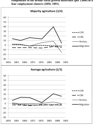
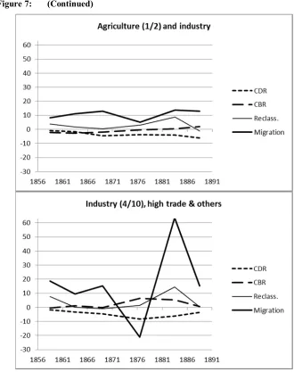
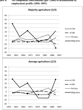
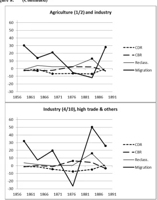
In the majority agricultural cluster the migration component always has a positive effect on urbanisation, with a peak in the recovery period (1881–1886) and a drop in the post-recovery period (1886–1991). Mortality does not differ much between urban and rural areas, while the fertility component contributes negatively to urbanisation in this cluster. However, in the recovery and post-recovery periods the gap between the mortality and fertility components shrinks, essentially because the contribution of fertility becomes less negative. In the average agricultural cluster the migration component is always positive, except in the post-war crisis period (1872–1881) when it is nil, while the recovery peak is visible but much less pronounced than in the majority agricultural cluster. Both the mortality and fertility components contribute negatively over the study period. In the half-agricultural cluster the migration component more or less follows the same trend as in the previous average agricultural cluster although the effect is less pronounced (the recovery peak is only visible if we take reclassification into account). The trend for the mortality and fertility components is almost the opposite to that for the majority agricultural cluster: starting at an almost equal level at the beginning of the study period they diverge with time, with the mortality component becoming more and more negative, while the fertility component is nil at the end of the post-recovery period. In the industrial and diversified cluster the migration component’s trend is very pronounced, with the only case of negative contribution occurring in the crisis period (1872–1881) and with a high peak in the recovery period (1881–1886) accentuated by reclassification. As for the natural components, they first diverge up to the crisis period, with mortality having a negative effect and fertility a positive one, and then converge, with fertility having a nil effect and mortality still having a slightly negative effect in the post-recovery period.
Figure 7: (Continued)
distance to main cities, rural density, and the availability of education (see methods section).
Figure 8: Net component contributions (per 1,000) to urbanisation by
Figure 8: (Continued)
Note: Estimates marked with a black dot are significantly different from 0; p-value<0.05
estimated components of urbanisation in each employment profile cluster and for each inter-census period, all other factors (urbanisation level, urbanisation of neighbouring counties, distance to Paris and large cities, rural density, availability of education) being equal. For convenience, we refer to the regression model results as the ‘net component of urbanisation,’ as opposed to the ‘gross component of urbanisation,’ which refers to the descriptive results (Figure 7) to which the margins are directly comparable.
The first remarkable regression result is that the net migration component of urbanisation is accentuated as compared to the descriptive results and shows a similar U-shape pattern across employment profiles. It declined steadily from 1856 and became negative in the crisis and recovery period, except in the industrial and diversified cluster. The general pattern for the recovery and post-recovery periods differs in the net and gross patterns. The gross migration component for all provincial France shows a peak in the recovery period which is only visible in the net migration component for the industrial and diversified cluster. For the other clusters the peak is actually observed for the net reclassification component, which we recall is mainly due to migration. Moreover, the level of the net migration component in the post-recovery period is comparable in all clusters (between 2% and 3%).
The second remarkable feature is that the net mortality and fertility components also differ from their gross counterparts. The pattern is also much more similar across clusters in the net than in the gross estimations. Generally, the urban penalty due to higher mortality in urban areas (as compared to rural areas) is not really apparent before 1866. Even during the post-war period of crisis and recovery (1872–1886), higher mortality is never compensated for by higher fertility in urban areas. The situation is reversed in the very last, post-recovery period (1886–1891): mortality benefits urban areas (there is no more urban penalty) while fertility is again detrimental to urban areas as in the pre-war period, particularly in the more agricultural county clusters.
1872) and by +0.04% (p<0.036) in the following crisis period for each 100 km. Distance to Paris increases the migration contribution to urbanisation in the 1861–1866 pre-war period (by +0.25% for each 100 km, p<0.014) and in the 1881–1886 recovery period (by +0.63% for each 100 km, p<0.036).
To sum up, the effect of greater distance to a large city is to reduce the natural components of urbanisation mainly in the crisis and recovery periods. This means that the pattern (an increased gap between the mortality and fertility components) observed in the crisis and recovery periods for the net natural components (Figure 7) is essentially associated with the counties hosting large cities or with the counties nearby. The distinctly negative mortality contribution and the slightly positive fertility contribution were therefore limited historically to the crisis and recovery periods and spatially to central counties (i.e., with large cities within reach), at a time when these counties attracted fewer migrants. In other words, the post-war negative net migration in these counties revealed the underlying negative effect of mortality (urban penalty) and positive effect of fertility.
We note that the effect of distance to Paris for the natural components of urbanisation is limited in time to before the employment structure variable is introduced into the model (negative effect on the fertility component after the war, positive effect on the mortality component during the war and crisis periods) and disappears after it is introduced (compare the results in Tables A-2 and A-3 in the Appendix). Also, the effect of distance to Paris on the migration component before the war is reduced after introducing the employment cluster variable. These cancelled or reduced effects mean that employment better explains variations in the migration, mortality, and fertility components of urbanisation than proximity to Paris. In fact, the effect of distance to large cities on the migration component remains almost unaffected by the introduction of the employment cluster variable.
In conclusion, in terms of distance to main cities, the effect of distance to Paris on natural components is mediated by the employment structure, while the migration component of urbanisation is strongly driven by the overall national political and economic situation and to a lesser extent by difference in employment structure. Although detailed migration data by origin and destination is lacking, our analysis leads us to assume that the post-war period led to a redistribution of long-distance migration previously oriented toward urbanised central counties to cities in less-urbanised (i.e., peripheral) counties. In the meantime, the population of central counties experienced an urban penalty not quite compensated for by a fertility advantage, possibly due to a higher proportion of reproductive-age population.
additional school for 10 municipalities; p<0.008), while it has no significant effect on the migration contribution. Similarly, rural density (push factor) is positively associated with the fertility contribution (+0.043% per additional rural inhabitant for 1,000 hectares; p<0.027) and is negatively associated with the mortality contribution (−0.063% per additional rural inhabitant for 1,000 hectares; p<0.0005), while it has no significant effect on the migration contribution. The effects of both availability of education and rural density do not differ before and after introducing the employment structure variable. It is worth noting that the negative association with mortality compensates for the positive association with fertility for both variables. Therefore, these factors have a net negative effect on the natural component of urbanisation while having no effect on the migration component – which is rather unexpected, since these factors were thought to push, or pull, population toward urban areas. Also, the effect of availability of education is counterintuitive, since its negative effect on the mortality component contributes to the urban penalty.
4. Discussion
Our analysis of the role of employment in the components of urbanisation at the county level in France has pointed to the crucial role played not so much by a particular component or sector of the economy but by the structure of a county’s economy and by the national political and economic context. The regression analysis using four clusters of counties according to their employment structures as determinants, controlling for urbanisation level and diffusion factors (urbanisation of neighbouring counties, distance to large cities and Paris) and for push and pull factors (rural density and availability of education), clearly shows the underlying urban penalty and period effects in the central counties (within reach of the largest cities) that were not apparent using descriptive statistics only. Results show how a shock (the 1870–1871 Franco-Prussian war and post-war crisis) affected urbanisation negatively through its migration component and probably redistributed migration temporarily towards smaller cities in peripheral counties. These results concur with those of Lerch and Stegemann (2017), who show how the business cycle and the political context affected internal and international migration to Zurich in the 19th and 20th centuries, and how Zurich’s population
As regards checking our initial hypotheses, results largely confirm that economic activity drives the urbanisation process through its migration component and not through its natural components. In the net component analysis the urban penalty (excess urban mortality) – confirmed found only between 1866 and 1886 (the war, crisis, and recovery periods) – is partially compensated for by higher urban fertility, and only marginally explains the slowdown in urbanisation, essentially in the most urbanised counties. Indeed, these natural component effects are not discernible in the gross component analysis. On the contrary, the net component analysis reveals that the 1870– 1871 shock and its aftermath explain variations in the migration component much more than those in the natural components of urbanisation. The reclassification component, which is driven mainly by migration, somewhat compensated for the direct migration component deficit during the recovery period. As in Belgium and Sweden, the overall direct and indirect contribution of migration to urbanisation by far exceeds the natural contribution before, and to an even greater degree after, controlling for the economic structure and other control variables. The results for the three countries contradict de Vries’ hypothesis that demographic transition drove the urban transition and concur with Zelinsky’s hypothesis that the redistribution of economic production, through mobility transition, drove the urban transition.
Conversely, our hypothesis regarding the geographical diffusion of the urban growth model from the centre (Paris) to the periphery (possibly through major cities) is not confirmed. The natural components of urbanisation are affected by distance to these cities only indirectly through the employment structure, which further confirms our previous hypothesis on the role of the economy in the urbanisation process. The migration component is only temporarily affected by distance, mainly to large cities during the crisis period and marginally to Paris in the recovery period, with migration presumably redistributed to smaller urban centres during these periods. The hierarchical dependence (interspace competition and centre–periphery hierarchy) does not act directly on urban transition by way of proximity to the centres of economic and political power (e.g., Paris and large cities) but essentially through the employment structure and the redistribution of migration.
because of a lack of ability on the part of the peasantry to seize urban opportunities but rather because of the lack of these opportunities. We add that the war and post-war crisis greatly contributed to this lack of urban opportunity.
The residual method used in this paper to evaluate the migration component has its limits. To better characterise the role of the migration component of urban transition, more detailed data on migration flows by origin and destination would be necessary. In particular, checking our assumption of redistribution of migration flows to the detriment of large cities during periods of crisis would require intra- versus inter-county migration data. Similarly, international net migration cannot be distinguished from internal net migration, as was done by Lerch and Stegemann (2017) for Zurich. Also, the effects of migration on sex and age structure cannot be assessed with the type of data used in this paper, although these effects may explain variations in the mortality and fertility components. For example, the change from male-dominated circular migration to permanent family migration over the 19th century (Châtelain 1967;
Kesztenbaum 2006) certainly had an impact on urban transition that the data at hand could not evaluate.
Beyond the analysis of historical French data, the modelling approach adopted in this paper could be applied to other contexts. The urban transition could be analysed in the same way at the international level, given data availability. The 19th-century French
References
Adams, J.J. (2017). Urbanization, long-run growth, and the demographic transition. Gainsville: University of Florida, Department of Economics (Unpublished working paper).
Bairoch, P. (1988).Cities and economic development: From the dawn of history to the
present. Chicago: University of Chicago Press.
Bairoch, P. (1996). Cinq millénaires de croissance urbaine. In: Sachs, I. (ed.). Quelles
villes, pour quel développement. Paris: Puf: 17‒60.
Bardet, J.-P. (1983).Rouen aux XVIIe et XVIIIe siècles. Paris: SEDES.
Bardet, J.-P. (1998). La France en déclin. In: Bardet, J.-P. and Dupâquier, J. (eds.). Histoire des populations de l’Europe: II. La révolution démographique, 1750‒ 1914. Paris: Fayard: 287–325.
Baudin, T. and Stelter, R. (2016). Rural exodus and fertility at the time of industrialization. Louvain-la-Neuve: Université catholique de Louvain, Institut de Recherches Économiques et Sociales (Discussion paper 2016-20).
https://sites.uclouvain.be/econ/DP/IRES/2016020.pdf.
Bocquier, P. (2005). World urbanization prospects: An alternative to the UN model of projection compatible with urban transition theory. Demographic Research 12(9): 197‒236.doi:10.4054/DemRes.2005.12.9.
Bocquier, P. (2015). The future of urban projections: Suggested improvements on the UN method.Spatial Demography 2(2): 1‒14.doi:10.1007/s40980-015-0005-1. Bocquier, P. and Costa, R. (2015). Which transition comes first? Urban and
demographic transitions in Belgium and Sweden. Demographic Research 33(48): 1297‒1332.doi:10.4054/DemRes.2015.33.48.
Brée, S. (2015). La population de la région parisienne au XIXe siècle.
Louvain-la-Neuve: Université catholique de Louvain, Centre de recherche en démographie (Working paper 6). https://cdn.uclouvain.be/public/Exports%20reddot/demo/ documents/Bree2sur1.pdf.
Brée, S. (2017).Paris l'inféconde: La limitation des naissances en région parisienne au
XIXe siècle. Paris: Ined Éditions.
Châtelain, A. (1967). Les migrations temporaires françaises au XIXe siècle: Problèmes,
Christiaensen, L., Gindelsky, M., and Jedwab, R. (2013). Rural push, urban pull or... urban push? New historical evidence from 40 developing countries. Silver Spring: Editorialexpress.com. https://editorialexpress.com/cgi-bin/conference/ download.cgi?db_name=NEUDC2013&paper_id=56.
de Vries, J. (1984).European urbanization, 1500‒1800. London: Methuen.
de Vries, J. (1990). Problems in the measurement, description, and analysis of historical urbanization. In: van der Woude, A., Yayami, A., and de Vries, J. (eds.).
Urbanization in history. Oxford: Clarendon Press: 43‒60.
Dormois, J.-P. (2005). Le visible et les invisibles: La productivité des services en France et en Angleterre au cours de l’industrialisation. Revue d’Histoire
Moderne et Contemporaine52(4): 152‒181.doi:10.3917/rhmc.524.0152.
Dyson, T. (2011). The role of the demographic transition in the process of urbanization.
Population and Development Review 37(1): 34‒54. doi:10.1111/j.1728-4457.
2011.00377.x.
Fox, S. (2012). Urbanization as a global historical process: Theory and evidence from sub-Saharan Africa. Population and Development Review 38(2): 285‒310.
doi:10.1111/j.1728-4457.2012.00493.x.
Garden, M. and Le Bras, H. (1988). La dynamique régionale. In: Dupâquier, J. (ed.).
Histoire de la population française: III. De 1789 à 1914. Paris: Puf: 138‒162.
Henderson, J.V., Roberts, M., and Storeygard, A. (2013). Is urbanization in sub-Saharan Africa different? Washington, D.C.: World Bank (Policy research working paper 6481).
Henry, L. (1967).Manuel de démographie historique. Paris: INED.
Heywood, C. (1981). The role of the peasantry in French industrialization, 1815–1880.
The Economic History Review 34(3): 359‒376.
Kesztenbaum, L. (2006). Une histoire d’espace et de patrimoine: Familles et migration dans la France de la Troisième République, 1870‒1940 [PhD thesis]. Paris: L’Institut d’Études Politiques.
Knodel, J. and Van de Walle, E. (1979). Lessons from the past: Policy implications of historical fertility studies. Population and Development Review5(2): 217‒245.
Lerch, M. and Stegemann, L. (2017).City growth in international perspective: The case
of industrializing Zurich 1760‒1949. Paper presented at the Population
Association of America Annual Meeting, Chicago, April 26‒29, 2017.
Lévy-Leboyer, M. and Bourguignon, F. (1985). L’économie française au XIXe siècle:
Analyse macro-économique. Paris: Éditions Économica.
Lhomme, J. (1970). La crise agricole à la fin du XIXe siècle en France: Essai
d’interprétation économique et sociale.Revue Économique 21(4): 521‒553. Marchand, O. and Thélot, C. (1997).Le travail en France, 1800–2000. Paris: Nathan. Motte, C. and Pelissier, J.-P. (1992). La binette, l’aiguille et le plumeau: Les mondes du
travail féminin. In: Dupâquier, J. and Kessler, D. (eds.).La société française au
XIXe siècle. Paris: Fayard: 237‒342.
Rollet, C. (1978). Allaitement, mise en nourrice et mortalité infantile en France à la fin du XIXe siècle.Population (French edition) 33(6): 1189‒1203.
Rollet, C. (1982). Nourrices et nourrissons dans le département de la Seine et en France de 1880 à 1940.Population (French edition) 37(3): 573‒604.
Schweitzer, S. (2002).Les femmes ont toujours travaillé: Une histoire du travail des
femmes aux XIXe et XXe siècles. Paris: Odile Jacob.
Sharlin, A. (1986). Urban‒rural differences in fertility in Europe during the demographic transition. In: Coale, A.J. and Watkins, S.C. (eds.). The decline of fertility in Europe: The revised proceedings of a conference on the Princeton
European Fertility Project. Princeton: Princeton University Press: 234‒260.
Statistiska Centralbyrån (1969). Historisk statistik för Sverige: Del 1: Befolkning, 2nd
edition, 1720‒1967. Stockholm: Statistiska Centralbyrån. https://www.scb.se/ Grupp/Hitta_statistik/Historisk_statistik/_Dokument/Historisk-statistik-for-Sverige-Del-1.pdf.
United Nations (2015). World urbanization prospects: The 2014 revision. New York: United Nations, Department of Economic and Social Affairs, Population Division.https://esa.un.org/unpd/wup/publications/files/wup2014-report.pdf. Zelinsky, W. (1971). The hypothesis of the mobility transition. The Geographical
Appendix
Figure A-1: Dendrogram justifying the clustering in four groups
Table A-1: Percentage distribution of male employment sectors in the four clusters (N=480 periods, 80 counties)
Cluster % agriculture % industry % commerce/transport % public sector % clergy % other Total (N=periods)
1. Majority agriculture 73.8 13.6 3.4 1.9 0.6 6.8 100.0
(91)
2. Average agriculture 63.2 19.2 5.1 2.5 0.6 9.5 100.0
(162)
3. Half agriculture 51.9 24.7 7.1 3.1 0.6 12.6 100.0
(144)
4. High industry 36.4 38.2 8.6 2.9 0.6 13.3 100.0
(83)
Provincial France 57.2 23.0 6.0 2.6 0.6 10.6 100.0
(480) 0 50 00 0 10 00 00 15 0 0 00 L2 sq u ar e d d is si m ila rit y m ea su re G 1 n= 1 9 G 2 n= 4 3 G 3 n= 2 9 G 4 n= 3 8 G 5 n= 6 3 G 6 n= 5 7 G 7 n= 4 G 8 n= 4 2 G 9 n= 3 0 G 10 n= 1 1 G 11 n= 4 6 G 12 n= 3 8 G 13 n= 2 6 G 14 n= 2 4 G 15 n= 1 0
Dendrogram for pward cluster analysis
Cluster 1 Cluster 2
Table A-2: Generalized structural equation model with period-cluster interactions (N = 480 periods, 80 counties)
Coef. Std. Err. z P>|z| [95% Conf. Interval]
Lower bound Upper bound ∆ Crude birth rate
Cluster 1 1856‒1861 ‒.1654252 .1255682 ‒1.32 0.188 ‒.4115344 .0806841
Cluster 2 1856‒1861 [REF]
Cluster 3 1856‒1861 .0329945 .0943973 0.35 0.727 ‒.1520209 .2180098
Cluster 4 1856‒1861 .1280603 .1184967 1.08 0.280 ‒.104189 .3603096
Cluster 1 1861‒1866 ‒.1240144 .2649766 ‒0.47 0.640 ‒.643359 .3953302
Cluster 2 1861‒1866 .0384582 .2303661 0.17 0.867 ‒.4130511 .4899675
Cluster 3 1861‒1866 ‒.01368 .2174963 ‒0.06 0.950 ‒.4399648 .4126048
Cluster 4 1861‒1866 .2960165 .2065524 1.43 0.152 ‒.1088188 .7008518
Cluster 1 1866‒1872 ‒.1856375 .2705722 ‒0.69 0.493 ‒.7159494 .3446744
Cluster 2 1866‒1872 ‒.170505 .2515587 ‒0.68 0.498 ‒.663551 .322541
Cluster 3 1866‒1872 .0533046 .2236453 0.24 0.812 ‒.3850322 .4916414
Cluster 4 1866‒1872 .1384245 .2158926 0.64 0.521 ‒.2847173 .5615662
Cluster 1 1872‒1881 .1678369 .3219953 0.52 0.602 ‒.4632622 .798936
Cluster 2 1872‒1881 .483464 .2781561 1.74 0.082 ‒.0617119 1.02864
Cluster 3 1872‒1881 .5257495 .2561125 2.05 0.040 .0237783 1.027721
Cluster 4 1872‒1881 .8993131 .3613527 2.49 0.013 .1910749 1.607551
Cluster 1 1881‒1886 .2862554 .386674 0.74 0.459 ‒.4716117 1.044122
Cluster 2 1881‒1886 .2285488 .294768 0.78 0.438 ‒.3491858 .8062834
Cluster 3 1881‒1886 .496352 .2641366 1.88 0.060 ‒.0213463 1.01405
Cluster 4 1881‒1886 .6883648 .3044544 2.26 0.024 .0916451 1.285085
Cluster 1 1886‒1891 ‒.6885634 .6139487 ‒1.12 0.262 ‒1.891881 .5147539
Cluster 2 1886‒1891 ‒.50412 .6189526 ‒0.81 0.415 ‒1.717245 .7090048
Cluster 3 1886‒1891 ‒.0048082 .3040705 ‒0.02 0.987 ‒.6007755 .591159
Cluster 4 1886‒1891 ‒.0797988 .2713408 ‒0.29 0.769 ‒.611617 .4520195
Percent Urban .0247967 .0095162 2.61 0.009 .0061453 .0434481
Percent Urban squared ‒.0004101 .0001511 ‒2.71 0.007 ‒.0007063 ‒.000114
% Urb adjac counties .0037916 .0044376 0.85 0.393 ‒.0049059 .0124892
distance Paris
1856‒1861 ‒.0047338 .0235859 ‒0.20 0.841 ‒.0509614 .0414937
1861‒1866 ‒.0036038 .0219502 ‒0.16 0.870 ‒.0466253 .0394178
1866‒1872 .0038029 .0224414 0.17 0.865 ‒.0401815 .0477872
1872‒1881 ‒.0399536 .0268423 ‒1.49 0.137 ‒.0925636 .0126563
1881‒1886 ‒.0186202 .0307296 ‒0.61 0.545 ‒.0788491 .0416087
1886‒1891 .0042508 .0358918 0.12 0.906 ‒.0660958 .0745974
distance big city
1856‒1861 .0111527 .068575 0.16 0.871 ‒.1232518 .1455571
1861‒1866 ‒.0369207 .0665469 ‒0.55 0.579 ‒.1673503 .0935089
1866‒1872 ‒.0270994 .0769634 ‒0.35 0.725 ‒.177945 .1237462
1872‒1881 ‒.1812427 .0919291 ‒1.97 0.049 ‒.3614205 ‒.001065
1881‒1886 ‒.1764769 .1038328 ‒1.70 0.089 ‒.3799854 .0270316
1886‒1891 .2147553 .2119198 1.01 0.311 ‒.2005999 .6301104
Schools / 10 municip. .0170286 .0088342 1.93 0.054 ‒.0002861 .0343433
Rural pop / 1000 ha .0434283 .0196405 2.21 0.027 .0049335 .081923
Table A-2: (Continued)
Coef. Std. Err. z P>|z| [95% Conf. Interval]
Lower bound Upper bound ∆ Crude death rate
Cluster 1 1856‒1861 .0777638 .13486 0.58 0.564 ‒.1865568 .3420845
Cluster 2 1856‒1861 [REF]
Cluster 3 1856‒1861 ‒.066307 .1081227 ‒0.61 0.540 ‒.2782236 .1456097
Cluster 4 1856‒1861 .0982287 .1394441 0.70 0.481 ‒.1750768 .3715342
Cluster 1 1861‒1866 .2993125 .2709317 1.10 0.269 ‒.2317038 .8303288
Cluster 2 1861‒1866 .0247931 .2455418 0.10 0.920 ‒.45646 .5060462
Cluster 3 1861‒1866 .0977549 .221865 0.44 0.659 ‒.3370926 .5326023
Cluster 4 1861‒1866 .0494554 .2321257 0.21 0.831 ‒.4055025 .5044134
Cluster 1 1866‒1872 ‒.2540974 .3157666 ‒0.80 0.421 ‒.8729886 .3647938
Cluster 2 1866‒1872 ‒.3295984 .2597944 ‒1.27 0.205 ‒.838786 .1795892
Cluster 3 1866‒1872 ‒.4638664 .253732 ‒1.83 0.068 ‒.961172 .0334391
Cluster 4 1866‒1872 ‒.252214 .2272658 ‒1.11 0.267 ‒.6976467 .1932188
Cluster 1 1872‒1881 ‒.1970892 .2749521 ‒0.72 0.473 ‒.7359854 .341807
Cluster 2 1872‒1881 ‒.5074536 .2356805 ‒2.15 0.031 ‒.9693788 ‒.0455283
Cluster 3 1872‒1881 ‒.4342873 .2137216 ‒2.03 0.042 ‒.853174 ‒.0154006
Cluster 4 1872‒1881 ‒.543145 .2476118 ‒2.19 0.028 ‒1.028455 ‒.0578348
Cluster 1 1881‒1886 ‒.2726892 .3965021 ‒0.69 0.492 ‒1.049819 .5044406
Cluster 2 1881‒1886 ‒.4297319 .3216814 ‒1.34 0.182 ‒1.060216 .200752
Cluster 3 1881‒1886 ‒.4883713 .2863986 ‒1.71 0.088 ‒1.049702 .0729596
Cluster 4 1881‒1886 ‒.2975623 .2548448 ‒1.17 0.243 ‒.7970489 .2019243
Cluster 1 1886‒1891 .7653373 .6553446 1.17 0.243 ‒.5191145 2.049789
Cluster 2 1886‒1891 .6708012 .6595832 1.02 0.309 ‒.6219581 1.96356
Cluster 3 1886‒1891 .2153687 .3141517 0.69 0.493 ‒.4003573 .8310947
Cluster 4 1886‒1891 .3055672 .2967438 1.03 0.303 ‒.27604 .8871744
Percent Urban ‒.0077857 .0098293 ‒0.79 0.428 ‒.0270507 .0114793
Percent Urban squared .0002324 .0001477 1.57 0.116 ‒.000057 .0005218
% Urb adjac counties .0049407 .0050883 0.97 0.332 ‒.0050322 .0149135
distance Paris
1856‒1861 .047596 .0239411 1.99 0.047 .0006723 .0945198
1861‒1866 .0216887 .0224829 0.96 0.335 ‒.0223769 .0657543
1866‒1872 .0639474 .0243348 2.63 0.009 .0162521 .1116428
1872‒1881 .0440995 .0209751 2.10 0.036 .0029891 .08521
1881‒1886 .0388692 .0304551 1.28 0.202 ‒.0208218 .0985601
1886‒1891 .0142486 .0366882 0.39 0.698 ‒.0576589 .0861561
distance big city
1856‒1861 .0596796 .0709658 0.84 0.400 ‒.0794108 .19877
1861‒1866 ‒.0153026 .0634783 ‒0.24 0.810 ‒.1397178 .1091126
1866‒1872 .0412033 .0715863 0.58 0.565 ‒.0991033 .1815099
1872‒1881 .1956568 .0511699 3.82 0.000 .0953656 .2959481
1881‒1886 .2207156 .1035501 2.13 0.033 .017761 .4236701
1886‒1891 ‒.3215843 .2210117 ‒1.46 0.146 ‒.7547592 .1115906
Schools / 10 municip. ‒.0243471 .0091175 ‒2.67 0.008 ‒.0422171 ‒.0064771
Rural pop / 1000 ha ‒.0631654 .0160716 ‒3.93 0.000 ‒.0946651 ‒.0316656
Table A-2: (Continued)
Coef. Std. Err. z P>|z| [95% Conf. Interval]
Lower bound Upper bound ∆ reclassification
Cluster 1 1856‒1861 .0896898 .2642186 0.34 0.734 ‒.4281691 .6075487
Cluster 2 1856‒1861 [REF]
Cluster 3 1856‒1861 .3943766 .2546289 1.55 0.121 ‒.1046868 .8934401
Cluster 4 1856‒1861 .8872359 .55471 1.60 0.110 ‒.1999758 1.974447
Cluster 1 1861‒1866 1.094 .5257926 2.08 0.037 .0634657 2.124535
Cluster 2 1861‒1866 .8553898 .5750227 1.49 0.137 ‒.271634 1.982414
Cluster 3 1861‒1866 .9116329 .5690643 1.60 0.109 ‒.2037126 2.026978
Cluster 4 1861‒1866 .6727732 .4705988 1.43 0.153 ‒.2495835 1.59513
Cluster 1 1866‒1872 .5766592 .4449643 1.30 0.195 ‒.2954547 1.448773
Cluster 2 1866‒1872 .6750248 .4419757 1.53 0.127 ‒.1912317 1.541281
Cluster 3 1866‒1872 .7679259 .4372718 1.76 0.079 ‒.0891111 1.624963
Cluster 4 1866‒1872 .5194262 .4402973 1.18 0.238 ‒.3435407 1.382393
Cluster 1 1872‒1881 .9664033 .5504798 1.76 0.079 ‒.1125173 2.045324
Cluster 2 1872‒1881 .4709725 .4970094 0.95 0.343 ‒.503148 1.445093
Cluster 3 1872‒1881 .7794926 .4605455 1.69 0.091 ‒.1231601 1.682145
Cluster 4 1872‒1881 .5881766 .4603025 1.28 0.201 ‒.3139996 1.490353
Cluster 1 1881‒1886 1.889066 1.006645 1.88 0.061 ‒.0839214 3.862053
Cluster 2 1881‒1886 1.392978 .8710599 1.60 0.110 ‒.3142685 3.100224
Cluster 3 1881‒1886 1.818112 .7697074 2.36 0.018 .3095132 3.326711
Cluster 4 1881‒1886 2.124597 .668647 3.18 0.001 .8140727 3.435121
Cluster 1 1886‒1891 ‒1.400426 .731886 ‒1.91 0.056 ‒2.834896 .0340447
Cluster 2 1886‒1891 .1635954 .5028271 0.33 0.745 ‒.8219276 1.149118
Cluster 3 1886‒1891 .1385355 .4617036 0.30 0.764 ‒.7663868 1.043458
Cluster 4 1886‒1891 .3708937 .4574247 0.81 0.417 ‒.5256421 1.26743
Percent Urban .0126507 .015347 0.82 0.410 ‒.0174289 .0427302
Percent Urban squared ‒.0004012 .0002842 ‒1.41 0.158 ‒.0009582 .0001558
% Urb adjac counties ‒.00061 .0101362 ‒0.06 0.952 ‒.0204766 .0192565
distance Paris
1856‒1861 .0567002 .0506774 1.12 0.263 ‒.0426255 .156026
1861‒1866 ‒.0328286 .0431042 ‒0.76 0.446 ‒.1173113 .0516542
1866‒1872 ‒.0017035 .0251541 ‒0.07 0.946 ‒.0510047 .0475976
1872‒1881 ‒.0205484 .0349952 ‒0.59 0.557 ‒.0891378 .0480409
1881‒1886 ‒.0774805 .0968958 ‒0.80 0.424 ‒.2673929 .1124318
1886‒1891 .0116552 .0421275 0.28 0.782 ‒.0709131 .0942236
distance big city
1856‒1861 .2514899 .205376 1.22 0.221 ‒.1510396 .6540195
1861‒1866 ‒.1507422 .1571349 ‒0.96 0.337 ‒.458721 .1572366
1866‒1872 ‒.1950826 .1001924 ‒1.95 0.052 ‒.3914561 .0012909
1872‒1881 .0812389 .1147508 0.71 0.479 ‒.1436685 .3061463
1881‒1886 ‒.1618614 .2823407 ‒0.57 0.566 ‒.7152391 .3915163
1886‒1891 .0614014 .0898663 0.68 0.494 ‒.1147334 .2375362
Schools / 10 municip. .0218989 .0137166 1.60 0.110 ‒.0049852 .048783
Rural pop / 1000 ha .0400915 .0297525 1.35 0.178 ‒.0182223 .0984052
Table A-2: (Continued)
Coef. Std. Err. z P>|z| [95% Conf. Interval]
Lower bound Upper bound ∆ net migration
Cluster 1 1856‒1861 .9095267 .5118097 1.78 0.076 ‒.0936019 1.912655
Cluster 2 1856‒1861 [REF]
Cluster 3 1856‒1861 ‒.0564019 .6047695 ‒0.09 0.926 ‒1.241728 1.128925
Cluster 4 1856‒1861 .1347456 .6324714 0.21 0.831 ‒1.104876 1.374367
Cluster 1 1861‒1866 ‒2.227832 1.246123 ‒1.79 0.074 ‒4.670189 .2145245
Cluster 2 1861‒1866 ‒2.042874 1.195334 ‒1.71 0.087 ‒4.385685 .2999369
Cluster 3 1861‒1866 ‒1.693692 1.177979 ‒1.44 0.150 ‒4.002489 .6151054
Cluster 4 1861‒1866 ‒2.339286 1.220463 ‒1.92 0.055 ‒4.731349 .0527773
Cluster 1 1866‒1872 ‒.8011493 1.317607 ‒0.61 0.543 ‒3.383612 1.781313
Cluster 2 1866‒1872 ‒1.001319 1.237552 ‒0.81 0.418 ‒3.426876 1.424239
Cluster 3 1866‒1872 ‒.9736172 1.194994 ‒0.81 0.415 ‒3.315763 1.368528
Cluster 4 1866‒1872 ‒1.11824 1.22422 ‒0.91 0.361 ‒3.517667 1.281186
Cluster 1 1872‒1881 ‒3.419126 2.001858 ‒1.71 0.088 ‒7.342697 .5044439
Cluster 2 1872‒1881 ‒4.642348 1.767501 ‒2.63 0.009 ‒8.106587 ‒1.17811
Cluster 3 1872‒1881 ‒3.598001 1.61871 ‒2.22 0.026 ‒6.770615 ‒.4253873
Cluster 4 1872‒1881 ‒5.742294 2.236839 ‒2.57 0.010 ‒10.12642 ‒1.35817
Cluster 1 1881‒1886 ‒2.839133 4.533051 ‒0.63 0.531 ‒11.72375 6.045484
Cluster 2 1881‒1886 ‒4.672846 3.899921 ‒1.20 0.231 ‒12.31655 2.970858
Cluster 3 1881‒1886 ‒4.275417 4.269766 ‒1.00 0.317 ‒12.644 4.093172
Cluster 4 1881‒1886 1.944015 2.483502 0.78 0.434 ‒2.92356 6.81159
Cluster 1 1886‒1891 ‒.8364938 3.366969 ‒0.25 0.804 ‒7.435633 5.762645
Cluster 2 1886‒1891 ‒.0911146 1.529541 ‒0.06 0.952 ‒3.088959 2.90673
Cluster 3 1886‒1891 ‒.2766608 1.529494 ‒0.18 0.856 ‒3.274413 2.721092
Cluster 4 1886‒1891 ‒.5059967 1.515864 ‒0.33 0.739 ‒3.477035 2.465042
Percent Urban ‒.0602644 .0686564 ‒0.88 0.380 ‒.1948285 .0742997
Percent Urban squared .0020079 .0013938 1.44 0.150 ‒.000724 .0047398
% Urb adjac counties .0112974 .0496234 0.23 0.820 ‒.0859627 .1085575
distance Paris
1856‒1861 ‒.0650265 .1601493 ‒0.41 0.685 ‒.3789134 .2488604
1861‒1866 .2452008 .099339 2.47 0.014 .0505 .4399016
1866‒1872 ‒.0020779 .1020498 ‒0.02 0.984 ‒.2020917 .197936
1872‒1881 .2661869 .1854035 1.44 0.151 ‒.0971974 .6295711
1881‒1886 .6326921 .3023745 2.09 0.036 .0400489 1.225335
1886‒1891 ‒.0059577 .1429847 ‒0.04 0.967 ‒.2862024 .2742871
dist big city
1856‒1861 ‒.5463065 .4369868 ‒1.25 0.211 ‒1.402785 .310172
1861‒1866 .3015861 .3485097 0.87 0.387 ‒.3814804 .9846525
1866‒1872 .5393763 .3271176 1.65 0.099 ‒.1017624 1.180515
1872‒1881 1.359529 .4937819 2.75 0.006 .3917347 2.327324
1881‒1886 1.501224 1.865829 0.80 0.421 ‒2.155734 5.158182
1886‒1891 .2829676 .4157035 0.68 0.496 ‒.5317963 1.097732
Schools / 10 municip. ‒.1129272 .0847796 ‒1.33 0.183 ‒.2790922 .0532377
Rural pop / 1000 ha .1392512 .119831 1.16 0.245 ‒.0956133 .3741157
Table A-2: (Continued)
Coef. Std. Err. z P>|z| [95% Conf. Interval]
Lower bound Upper bound Variance
var(∆CBR) .2628566 .0682096 .1580658 .4371194
var(∆CDR) .2590221 .0759554 .1457911 .4601956
var(∆reclass.) .8826424 .1272297 .6654068 1.170799
var(∆net migr.) 12.35503 4.570043 5.983982 25.50924
Covariance
cov(∆CDR,∆CBR) ‒.2185164 .0711843 ‒3.07 0.002 ‒.3580351 ‒.0789978
cov(∆reclass.,∆CBR) ‒.0828209 .0216875 ‒3.82 0.000 ‒.1253277 ‒.0403142
cov(∆net mig.,∆CBR) ‒.1625766 .2689682 ‒0.60 0.546 ‒.6897447 .3645914
cov(∆reclass.,∆CDR) .0800233 .0201158 3.98 0.000 .0405971 .1194495
cov(∆net mig.,∆CDR) .1563931 .2996785 0.52 0.602 ‒.4309661 .7437522