VOLUME 36, ARTICLE 37, PAGES 1081−1108
PUBLISHED 5 APRIL 2017
http://www.demographic-research.org/Volumes/Vol36/37/ DOI: 10.4054/DemRes.2017.36.37
Descriptive Finding
The population-level impact of public-sector
antiretroviral therapy rollout on adult mortality
in rural Malawi
Collin F. Payne
Hans-Peter Kohler
© 2017 Collin F. Payne & Hans-Peter Kohler.
This open-access work is published under the terms of the Creative Commons Attribution NonCommercial License 2.0 Germany, which permits use, reproduction & distribution in any medium for non-commercial purposes, provided the original author(s) and source are given credit.
1 Background 1082
2 Methods 1083
2.1 Study design and participants 1083
2.2 Statistical analysis 1085
3 Results 1086
3.1 Pre-ART/post-ART differences in overall life expectancy 1086 3.2 Pre-ART/post-ART differences in mortality 1088
4 Discussion 1090
5 Acknowledgments 1091
References 1092
The population-level impact of public-sector antiretroviral therapy
rollout on adult mortality in rural Malawi
Collin F. Payne1 Hans-Peter Kohler2
Abstract
BACKGROUND
Recent evidence from health and demographic surveillance sites (HDSS) has shown that increasing access to antiretroviral therapy (ART) is reducing mortality rates in sub-Saharan Africa (SSA). However, due to limited vital statistics registration in many of the countries most affected by the HIV/AIDS epidemic, there is limited evidence of the magnitude of ART’s effect outside of specific HDSS sites. This paper leverages longitudinal household/family roster data from the Malawi Longitudinal Survey of Families and Health (MLSFH) to estimate the effect of ART availability in public clinics on population-level mortality based on a geographically dispersed sample of individuals in rural Malawi.
OBJECTIVE
We seek to provide evidence on the population-level magnitude of the ART-associated mortality decline in rural Malawi and confirm that this population is experiencing similar declines in mortality as those seen in HDSS sites.
METHODS
We analyze longitudinal household/family-roster data from four waves of the MLSFH to estimate mortality change after the introduction of ART to study areas. We analyze life expectancy using the Kaplan–Meier estimator and examine how the mortality hazard changed over time by individual characteristics with Cox regression.
RESULTS
In the four years following rollout of ART, life expectancy at age 15 increased by 3.1 years (95% CI 1.1, 5.1), and median length of life rose by over ten years.
1
Corresponding author: Center for Population and Development Studies, Harvard T.H. Chan School of Public Health. 9 Bow St, Cambridge, MA 02139. E-Mail:[email protected].
2
CONTRIBUTION
Our observations show that the increased availability of ART resulted in a substantial and sustained reversal of mortality trends in SSA and assuage concerns that the post-ART reversals in mortality are not occurring at the same magnitude outside of specific HDSSs.
1. Background
While life expectancy in the rest of the world continued to increase from the late 1980s through the 2000s, much of southern and eastern sub-Saharan Africa (SSA) saw reductions in life expectancy associated with the HIV pandemic (WHO 2014). Beyond the simple loss of life, these declines in life expectancy have had negative impacts on child survival, household income, availability of skilled labor, and work efforts (Barnett and Whiteside 2006). The large-scale rollout of antiretroviral therapy (ART) in SSA has begun to reverse these trends (Joint United Nations Programme on HIV/AIDS (UNAIDS) 2013). ART works by enabling an individual’s immune system to recover to a functional state and can improve survival to levels almost on par with those of the non-HIV infected (Mills et al. 2011). Starting in the early 2000s, access to ART through public-sector programs was greatly improved in SSA. Recent studies have started to document the success of these programs in terms of population-level declines in mortality (both HIV-related and all-cause) in South Africa (Bor et al. 2013; Larson et al. 2014), Malawi (Floyd et al. 2010; Jahn et al. 2008; Price et al. 2016), and other countries in SSA (Floyd et al. 2012; Stoneburner et al. 2014).
comparison), it is nevertheless possible and plausible that the observed ART-related mortality reductions in HDSS sites represent a more ideal case than exists in much of SSA.
In this paper, we use an alternative approach and data source to estimate the effect of ART introduction on population-level mortality. Namely, we estimate the effect of ART availability in public clinics on population-level mortality based on a geographically dispersed, mostly rural sample of individuals from the Malawi Longitudinal Study of Families and Health (MLSFH; Kohler et al. 2015), which reflects substantial heterogeneity in ethnicity, religion, language, educational attainment, population density, and HIV prevalence.
Besides the comparison with related estimates from HDSS sites, our findings about pre- and post-ART mortality are key for documenting recent mortality levels and trends in the MLSFH. This study population is a publicly available, ongoing cohort study that has been used in more than 250 publications.3 Our finding that the mortality of the MLSFH study population is similar, in both level and trends, to that documented in other HDSS sites strengthens the assessment of data quality in the MLSFH, highlights an innovative new use of the MLSFH data based on linked household/family-roster data, and provides additional credence to the ongoing relevance of the MLSFH for studying contemporary trends in demographic, health, and social conditions in SSA.
2. Methods
2.1 Study design and participants
We estimate age-specific mortality among respondents and household/family members
in the 2004‒2012 MLSFH. The MLSFH is a longitudinal study monitoring social,
economic, and health conditions in the rural population of Malawi, one of the world’s poorest nations. The study is based in three rural districts (Rumphi in the north, Mchinji in the center, and Balaka in the south; Figure A-1) that represent the substantial heterogeneity of Malawi in terms of HIV prevalence and ethnic/religious groups (Kohler et al. 2015). MLSFH respondents (N≈3,800) are evenly split among these three regions and are clustered in 121 villages. MLSFH sampling methods and related data collection procedures are described in a cohort profile (Kohler et al. 2015). Comparisons with the nationally representative Malawi Demographic and Health Surveys and the Malawi Third Integrated Household Survey show that basic
demographic characteristics closely match the rural population of Malawi (Kohler et al. 2015; Payne, Mkandawire, and Kohler 2013).
At each wave, MLSFH respondents reported on the mortality of their resident and nonresident household/family members. The MLSFH offered HIV testing and counseling services to primary respondents and their spouses in 2004, 2006, and 2008, with referral to confirmatory testing at a local clinic for those with HIV+ results (Kohler et al. 2015). The survey team did not interact directly with other members of the household roster, who comprise about 70% of the individuals in this study. The MLSFH also had no part in the training, support, or management of ART provision, making the study population independent from the ART program that is being evaluated in terms of its effect on population-level mortality.
The Ministry of Health in Malawi began rolling out free ART to eligible individuals in urban areas in 2004, with rollout to smaller clinics beginning in 2006. In the MLSFH, median distance of respondents to the nearest ART clinic was 27 kilometers up until mid-2007, which made access to ART difficult given the limited means of transportation in this rural context (Baranov, Bennett, and Kohler 2015; Baranov and Kohler 2014). ART-providing clinics opened between August of 2007 and March of 2008 in each of the three study regions (shortly before data collection for the 2008 round of the MLSFH), reducing the median distance to the nearest ART clinic to 8.9 kilometers by the 2008 MLSFH (Baranov, Bennett, and Kohler 2015).
HIV prevalence among MLSFH respondents was 6.1% in 2010, with considerable variation across regions (Freeman and Anglewicz 2012). It was higher among men age 50‒65 (8.9%) than women age 50‒65 (5.4%), but lower among men age 15‒49 (4.1%) than women age 15‒49 (8.3%).
The study population consists of (a) MLSFH respondents and (b) individuals who were reported on the MLSFH household/family rosters by respondents in 2004, 2006, 2008, 2010, and 2012. However, the 2004 household roster questionnaire used a different inclusion criterion (only recording members who slept in the household the previous night), so our primary results will focus on the 2006‒2012 MLSFH. In each wave, primary respondents completed a family and household roster listing the vital status of their family/household members independent of place of residence (more detail on the household/family rosters and the full set of questions asked in the roster module is included in Appendix Text 1).
Individuals reported on the MLSFH family/household roster were not previously linked across survey rounds to allow longitudinal analyses. We developed a probabilistic matching algorithm to link individuals across multiple MLSFH waves by name, age, sex, and relationship to primary respondent (see Appendix Text 2 for details
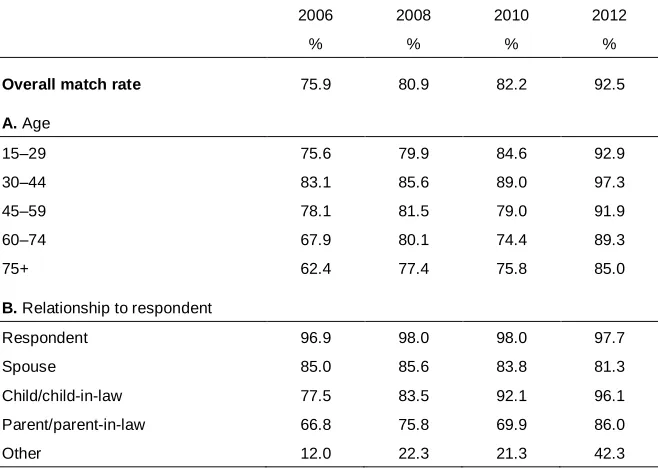
on the matching process). Match rates between successive waves were 76‒82% in
2006‒2010 and 92% in 2012, with rates for close family members (parents, children, spouses) substantially higher. The higher match rate in 2012 resulted from the fact that household rosters were prepopulated with information from the 2010 survey. Failure to link is unlikely to introduce biases in our analyses (see Appendix Tables A-1 and A-2).
Our analysis population included all resident and nonresident family/household members aged 15 and older (including the respondent themselves) who were linked across at least two survey waves. To avoid duplicate records resulting from both husband and wife reporting on the same family/household members, we limited our analysis sample to individuals listed by female primary respondents and male respondents without a coresident spouse in the MLSFH sample. With these restrictions, our analyses sample consists of 9,586 individuals listed by 1,869 primary MLSFH respondents, contributing 33,103 person years of observation during the period 2006‒ 2012. Appendix Table A-2 presents selected characteristics of the analytic sample. A total of 735 deaths were observed in the study population between 2006 and 2012.
2.2 Statistical analysis
Age-specific mortality rates are computed for pre-ART (2006‒2008) and post-ART
(2008‒2010, 2010‒2012) periods. Trends in pre-ART and post-ART survival curves
with 95% confidence intervals are estimated using the Kaplan–Meier estimator (Kalbfleisch and Prentice 2002), and adult life expectancies were obtained as the area under the survival curve after age 15. Adult life expectancy measures the additional years a 15-year-old would expect to live if subjected to the prevailing pattern of mortality rates in the population. We also report the median length of life conditional on survival to age 15 as the age at which the survival curve for each period reached .5.
To increase analytic power, we compared data from 2006‒2008 (pre-ART period)
to combined 2008‒2010 and 2010‒2012 data (post-ART period). Analyses used
vs. 8 or more kilometers), completed primary schooling (fewer than five years of completed schooling vs. five or more years completed schooling), and quartiles of
household wealth (measured via an asset index and averaged over the period 2006‒
2012).
3. Results
3.1 Pre-ART/post-ART differences in overall life expectancy
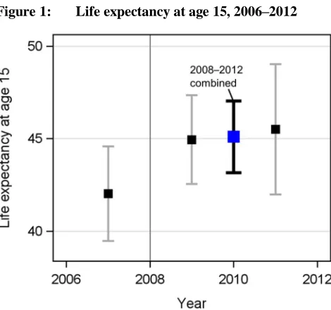
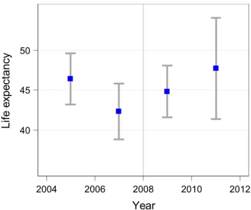
Figure 1 shows that adult life expectancy (LE at age 15) before the introduction of ART (period 2006‒2008) was approximately 42 years in the study population (95% CI 39.4, 44.6) – slightly below the 2010 GBD estimates for adult life expectancy in Malawi, 43.2 years (Salomon et al. 2012). Adult life expectancy increased to approximately 45 years (95% CI 42.5, 47.4) in the period directly after the introduction of ART (2008‒ 2010). It was slightly higher, at 45.5 years (95% CI 41.9, 49.1), in the following period (2010‒2012). The difference in life expectancy between the pre-ART and the post-ART
period (2008‒2012 combined, LE 45.1 years, 95% CI 43.1, 47.1) was 3.1 years (95%
CI 1.1, 5.1). Life expectancies and 95% CIs for men and women separately are provided in Appendix Table A-3. Sensitivity analyses using alternative definitions of the study population led to similar results (see Appendix Table A-4). Appendix Figure A-2 replicates Figure 1, including the 2004 MLSFH data and using a restricted sample
of individuals in the 2006‒2012 surveys to correspond to the household listing
Figure 1: Life expectancy at age 15, 2006‒2012
Notes: Life expectancy at age 15 is the mean length of remaining life for a 15-year-old if subjected to the prevailing pattern of age-specific mortality rates observed during a given period of time. Estimates of life expectancy for the periods 2006‒2008, 2008‒2010, and 2010‒2012 are displayed as the squares, with 95% CIs. The timing of public-sector introduction of ART is shown using the gray vertical line.
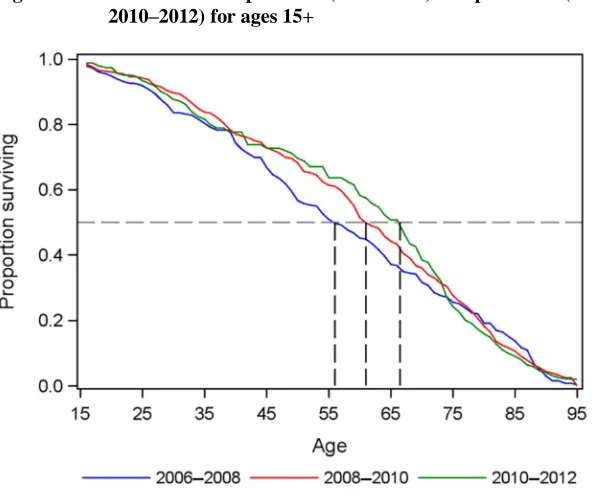
Comparing the survival curves of the pre-ART and post-ART periods (Figure 2), the median length of life conditional on survival to age 15 rose by 11 years between 2006 and 2012, from 56 years (95% CI 51, 62) before the introduction of ART to 61 years (95% CI 59, 65) in the period directly after the introduction of ART (2008‒2010)
and to 67 years (95% CI 60, 70) in 2010‒2012. For the post-ART period combined
Figure 2: Survival curves pre-ART (2006‒2008) and post-ART (2008‒2010, 2010‒2012) for ages 15+
Notes: Survival curves for pre-ART (2006‒2008, blue line) and post-ART (2008‒2010, red line, and 2010‒2012, green line) periods. Conditional on survival to age 15, median age at death was 56 years before the introduction of ART, rising after the introduction of ART to 61 years in 2008–2010 and 67 years in 2010–2012.
3.2 Pre-ART/post-ART differences in mortality
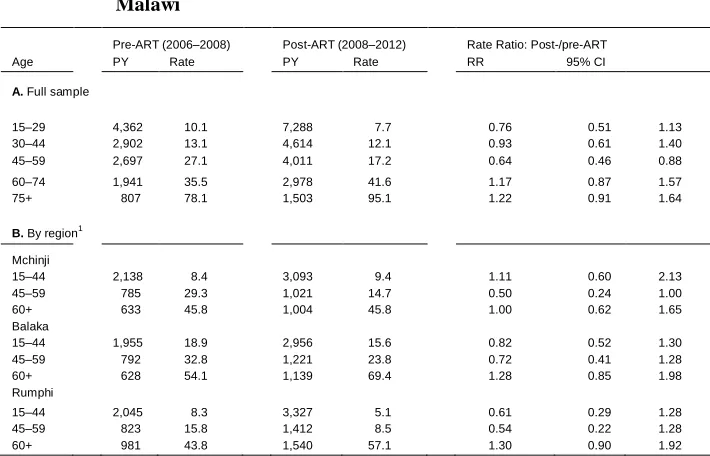
The all-cause mortality rate among those aged 15‒59 declined by almost 30% between the pre-ART and post-ART periods (from 15.6 to 11.4 deaths per thousand, RR .73, 95% CI .59, .91), with the strongest declines in the 45‒59 age group (Panel A of Table 1). At advanced ages (60+) these reductions subside.
Table 1: Trends in mortality before and after introduction of ART to rural Malawi
Pre-ART (2006‒2008) Post-ART (2008‒2012) Rate Ratio: Post-/pre-ART Age PY Rate PY Rate RR 95% CI A.Full sample
15‒29 4,362 10.1 7,288 7.7 0.76 0.51 1.13 30‒44 2,902 13.1 4,614 12.1 0.93 0.61 1.40 45‒59 2,697 27.1 4,011 17.2 0.64 0.46 0.88 60‒74 1,941 35.5 2,978 41.6 1.17 0.87 1.57 75+ 807 78.1 1,503 95.1 1.22 0.91 1.64
B. By region1 Mchinji
15‒44 2,138 8.4 3,093 9.4 1.11 0.60 2.13 45‒59 785 29.3 1,021 14.7 0.50 0.24 1.00 60+ 633 45.8 1,004 45.8 1.00 0.62 1.65 Balaka
15‒44 1,955 18.9 2,956 15.6 0.82 0.52 1.30 45‒59 792 32.8 1,221 23.8 0.72 0.41 1.28 60+ 628 54.1 1,139 69.4 1.28 0.85 1.98 Rumphi
15‒44 2,045 8.3 3,327 5.1 0.61 0.29 1.28 45‒59 823 15.8 1,412 8.5 0.54 0.22 1.28 60+ 981 43.8 1,540 57.1 1.30 0.90 1.92
1
Analyses by region use only individuals reported as primarily residing within that region.
Table 2: Cox hazard ratio estimates for distance from ART clinic, sex, education, and wealth pre-ART and post-ART
Pre-ART (2006‒2008) Post-ART (2008‒2012) Estimate 95% CI Estimate 95% CI Distance to ART clinic
8 kilometers or more ref ref
fewer than 8 kilometers 1.06 [0.79, 1.41] 0.77* [0.62, 0.97] Sex
Female ref ref
Male 1.74** [1.34, 2.26] 1.42** [1.16, 1.73] Education
Fewer than five years of
schooling ref ref
Five or more years of schooling 0.97 [0.72, 1.30] 0.86 [0.68, 1.10] Wealth quantile
1st ref ref
2nd 0.70+ [0.48, 1.03] 0.78 [0.58, 1.06] 3rd 0.76 [0.52, 1.10] 0.72* [0.52, 0.98] 4th 0.77 [0.52, 1.14] 0.75+ [0.54, 1.03] 5th 0.58* [0.38, 0.90] 0.75+ [0.54, 1.05]
Notes: Analyses additionally control for region and age, and they account for clustering within household. +p < 0.10*p< 0.05**p < 0.01
4. Discussion
We document gains of 3.1 years in adult life expectancy and 8 years of median length of life in the four years following the introduction of public-sector ART in rural Malawi. Our estimated mortality rates and the change in mortality rate post-ART are similar to published results from the Karonga HDSS in Malawi (Floyd et al. 2010; Larson et al. 2014; Price et al. 2016) and those of other HDSS sites in Southern and Eastern Africa (Floyd et al. 2012).
Although the increase in life expectancy coincided with the scale-up of ART (Figure 1 and Appendix Figure A-2), our estimates may also capture health and mortality trends not linked to the scale-up of ART. As there is no counterfactual group in our analyses, we cannot directly identify the causal mechanism behind the observed mortality declines. However, the coincidence of life expectancy increasing directly after the introduction of ART strongly suggests that the increased availability of ART was the primary driver. Few other health interventions addressing major causes of death occurred in rural Malawi during this time, and overall socioeconomic changes in Malawi were more likely to change mortality in the opposite direction, as the post-ART period coincided with substantial rises in food and oil prices, currency devaluation, political unrest, and reduced international aid (Ellis and Manda 2012; Wroe 2012).
Our analyses demonstrate the promise of using alternative data sources to add to the evidence base on the population-level effects of ART on mortality and life expectancy. Our results further support the assumption that the increased availability of ART resulted in a substantial and sustained reversal of mortality trends in rural Malawi and help assuage concerns that the post-ART reversals in mortality may not be occurring at the same magnitude outside of specific HDSSs. Future research will have to address the long-term consequences of ART on lifecycle behaviors among families affected by HIV and the possible economic benefits resulting from sustained health improvements through ART. Challenges in achieving high ART uptake and ART adherence among the rapidly growing population of older individuals with HIV will have to be addressed.
5. Acknowledgments
References
Asiki, G., Murphy, G., Nakiyingi-Miiro, J., Seeley, J., Nsubuga, R.N., Karabarinde, A., and GPC team (2013). The general population cohort in rural south-western Uganda: A platform for communicable and non-communicable disease studies. International Journal of Epidemiology 42(1): 129–141.doi:10.1093/ije/dys234.
Baranov, V., Bennett, D., and Kohler, H.-P. (2015). The indirect impact of antiretroviral therapy: Mortality risk, mental health, and HIV-negative labor supply. Journal of Health Economics 44: 195–211.doi:10.1016/j.jhealeco.2015.07.008.
Baranov, V. and Kohler, H.-P. (2014). The impact of AIDS treatment on savings and human capital investment in Malawi. Philadelphia: University of Pennsylvania Libraries (PSC Working Paper Series). http://repository.upenn.edu/ psc_working_papers/55/.
Barnett, T. and Whiteside, A. (2006). AIDS in the twenty-first century: Disease and
globalization (2nd ed.). Basingstoke: Palgrave Macmillan.
Bor, J., Herbst, A.J., Newell, M.-L., and Bärnighausen, T. (2013). Increases in adult life expectancy in rural South Africa: Valuing the scale-up of HIV treatment. Science339(6122): 961‒965.doi:10.1126/science.1230413.
Ellis, F. and Manda, E. (2012). Seasonal food crises and policy responses: A narrative
account of three food security crises in Malawi. World Development 40(7):
1407–1417.doi:10.1016/j.worlddev.2012.03.005.
Floyd, S., Marston, M., Baisley, K., Wringe, A., Herbst, K., Chihana, M., and Zaba, B. (2012). The effect of antiretroviral therapy provision on all-cause, AIDS and non-AIDS mortality at the population level: A comparative analysis of data from four settings in Southern and East Africa. Tropical Medicine and International Health17(8): e84–93.doi:10.1111/j.1365-3156.2012.03032.x.
Floyd, S., Molesworth, A., Dube, A., Banda, E., Jahn, A., Mwafulirwa, C., and French, N. (2010). Population-level reduction in adult mortality after extension of free anti-retroviral therapy provision into rural areas in Northern Malawi. PLoS One 5(10): e13499.doi:10.1371/journal.pone.0013499.
Freeman, E. and Anglewicz, P. (2012). HIV prevalence and sexual behaviour at older
ages in rural Malawi. International Journal of STD and AIDS 23(7): 490–496.
doi:10.1258/ijsa.2011.011340.
evidence of reversal after introduction of antiretroviral therapy in Malawi. Lancet371(9624): 1603–1611.doi:10.1016/S0140-6736(08)60693-5.
Joint United Nations Programme on HIV/AIDS (UNAIDS) (2013). UNAIDS report on the global AIDS epidemic 2013. Geneva: UNAIDS.
Kalbfleisch, J.D. and Prentice, R.L. (2002).The statistical analysis of failure time data (2nd ed.). Hoboken: Wiley-Interscience.doi:10.1002/9781118032985.
Kasamba, I., Baisley, K., Mayanja, B.N., Maher, D., and Grosskurth, H. (2012). The impact of antiretroviral treatment on mortality trends of HIV-positive adults in
rural Uganda: A longitudinal population-based study, 1999–2009. Tropical
Medicine and International Health 17(8): e66–e73.
doi:10.1111/j.1365-3156.2012.02841.x.
Kohler, H.-P., Watkins, S.C., Behrman, J.R., Anglewicz, P., Kohler, I.V., Thornton, R. L., and Kalilani-Phiri, L. (2015). Cohort profile: The Malawi Longitudinal Study
of Families and Health (MLSFH).International Journal of Epidemiology 44(2):
394–404.doi:10.1093/ije/dyu049.
Larson, E., Bendavid, E., Tuoane-Nkhasi, M., Mbengashe, T., Goldman, T., Wilson, M., and Klausner, J.D. (2014). Population-level associations between antiretroviral therapy scale-up and all-cause mortality in South Africa. International Journal of STD and AIDS 25(9): 636–642.doi:10.1177/09564624 13515639.
Mills, E.J., Bakanda, C., Birungi, J., Chan, K., Ford, N., Cooper, C. L., and Hogg, R.S. (2011). Life expectancy of persons receiving combination antiretroviral therapy
in low-income countries: A cohort analysis from Uganda. Annals of Internal
Medicine 155(4): 209–216.doi:10.7326/0003-4819-155-4-201108160-00358.
Mwagomba, B., Zachariah, R., Massaquoi, M., Misindi, D., Manzi, M., Mandere, B.C., and Harries, A.D. (2010). Mortality reduction associated with HIV/AIDS care and antiretroviral treatment in rural Malawi: Evidence from registers, coffin sales and funerals.PloS One 5(5): e10452.doi:10.1371/journal.pone.0010452.
Odhiambo, F.O., Laserson, K.F., Sewe, M., Hamel, M.J., Feikin, D.R., Adazu, K., and Vulule, J.M. (2012). Profile: The KEMRI/CDC Health and Demographic
Surveillance System ‒ Western Kenya. International Journal of Epidemiology
41(4): 977–987.doi:10.1093/ije/dys108.
Pillay-van Wyk, V., Msemburi, W., Laubscher, R., Dorrington, R.E., Groenewald, P., Matzopoulos, R., and Bradshaw, D. (2013). Second National Burden of Disease
Study South Africa: National and subnational mortality trends, 1997–2009. The
Lancet381(2): S113.doi:10.1016/S0140-6736(13)61367-7.
Price, A.J., Glynn, J., Chihana, M., Kayuni, N., Floyd, S., Slaymaker, E., and Crampin, A.C. (2016). Sustained 10-year gain in adult life expectancy following antiretroviral therapy roll-out in rural Malawi: July 2005 to June 2014. International Journal of Epidemiology.doi:10.1093/ije/dyw208.
Salomon, J.A., Wang, H., Freeman, M.K., Vos, T., Flaxman, A.D., Lopez, A.D., and Murray, C.J.L. (2012). Healthy life expectancy for 187 countries, 1990‒2010: A
systematic analysis for the Global Burden Disease Study 2010. Lancet
380(9859): 2144–2162.doi:10.1016/S0140-6736(12)61690-0.
Stoneburner, R., Korenromp, E., Lazenby, M., Tassie, J.-M., Letebele, J., Motlapele, D., and Low-Beer, D. (2014). Using health surveillance systems data to assess the impact of AIDS and antiretroviral treatment on adult morbidity and mortality in Botswana.PloS One 9(7): e100431.doi:10.1371/journal.pone.0100431.
Stover, J., Fidzani, B., Molomo, B.C., Moeti, T., and Musuka, G. (2008). Estimated
HIV trends and program effects in Botswana. PloS One 3(11): e3729.
doi:10.1371/journal.pone.0003729.
Tanser, F., Hosegood, V., Bärnighausen, T., Herbst, K., Nyirenda, M., Muhwava, W., and Newell, M.-L. (2008). Cohort profile: Africa Centre Demographic
Information System (ACDIS) and population-based HIV survey. International
Journal of Epidemiology 37(5): 956–962.doi:10.1093/ije/dym211.
Wambura, M., Urassa, M., Isingo, R., Ndege, M., Marston, M., Slaymaker, E., and Zaba, B. (2007). HIV prevalence and incidence in rural Tanzania: Results from
10 years of follow-up in an open-cohort study. Journal of Acquired Immune
Deficiency Syndromes46(5): 616–623.doi:10.1097/QAI.0b013e31815a571a.
WHO (2014). World health statistics 2014. Geneva: World Health Organization. http://public.eblib.com/choice/publicfullrecord.aspx?p=1741840.
Appendix Text 1: MLSFH household roster details
Beginning in 2006 and continuing in the 2008, 2010, and 2012 MLSFH waves, the MLSFH collected data on family structure. The MLSFH household and family roster included not only all individuals who currently live in the household (as frequently done in other studies), but it also asked for information about all parents, spouses (and the most recently deceased or divorced spouse for those not currently married), and children independent of their survival and resident status (Box 1).
Box 1:
Individuals listed in MLSFH household/family roster
1. List the respondent
2. List name of spouse(s) of respondent. If respondent is not currently married, list name of most recently deceased or divorced spouse. For polygamous men: List all wives. If never married, proceed to instruction 3, below.
3. List name of respondents’ parents (list names even if parents are deceased).
4. [if R is married or widowed] List name of spouse’s parents (list names even if parents are deceased). For polygamous men: List parents of all wives. 5. List the names of all children of the respondent (children ever born; include
children who are no longer alive or do not live in respondent’s household).
6. List the names of any other children who usually live in this household (including nonbiological children, grandchildren, nieces and nephews). 7. List the names of all other persons who slept in this household last night.
8. List the names of all other persons who usually sleep in this household but did not last night.
9. List the names of all nonrelated children who are under your care but not living in the household (for example, anyone you have helped with school fees in the last five years).
Box 2:
Information about each person listed on the MLSFH
household/family roster
Q2 What is [name’s] relationship to you?
Q3 Is [name] male or female?
Q4 Is [name] alive? If [name] is dead, when did he/she die? (Note:Questions Q5–
16 were not asked for persons who had died.)
Q5 How old is [name]? Or in what year was [name] born?
Q6 Where does [name] usually live?
Q7 Did [name] sleep here last night?
Q8 If a person does not regularly live here: When did [name] move to this place?
Q9 Has [name] been ill in the past 12 months? If yes, for how long?
Q10 How would you rate [name’s] health in general?
Q11 How would you compare [name’s] health to other people in your village who
are the same age and sex?
Q12 What is [name’s] current marital status?
Q13– 14
What is the highest level of schooling [name] completed? How many grades (in years) did [name] complete at that level?
Q15 If age>10: What is [name’s] main way of earning money?
Appendix Text 2: The matching process and diagnostics
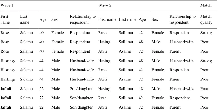
We developed a probabilistic matching algorithm that generated longitudinal links between individuals on the household rosters across rounds of data collection. Individuals are matched based on name, age, sex, and familial relationship to respondent. To illustrate the matching process, we use two waves of data on a hypothetical household roster (the Salamu family) as an example.
Wave 1:
First name Last name Age Sex Relationship to
respondent
Rose Salamu 40 Female Respondent
Hastings Salamu 44 Male Husband/wife
Jaffali Asamu 22 Male Son/daughter
Wave 2:
First name Last name Age Sex Relationship to
respondent
Rose Sallumu 42 Female Respondent
Hasing Sallumu 48 Male Husband/wife
Abiti Sallumu 72 Female Parent
On the surface, we see that the first two individuals on each roster are a likely match, although there are some minor spelling differences in the names provided. The third individuals on each roster do not appear to be a strong match. Our algorithm initially sorts each dataset by primary respondent, and within each primary respondent by the listed members of the household. We then generate a dataset of all possible permutations of wave 1 to wave 2 matches within each primary respondent (that is, a file with one data line for each possible combination of individuals reported on the household roster within each primary respondent).
Matching on name accounts for roughly half of the match score, while matching on age, sex, and relationship to respondent evenly account for the remainder of the match score. A match is counted as strong if the same individual is ranked first in each ranking (that is, the match has the highest score of all matches for each individual) and has a match score of over 65%. Lower-ranking matches (between 50% and 65%, or not ranking first across the same individual) are then set aside, cleaned of individuals with a strong match, and rematched using a higher threshold of 70%. This second match accounts for 1% or fewer of matched individuals. At this point, individuals with a match score of over 60%, or those who had a match score of over 50% but are missing information on one of the variables used in matching, are set aside for hand coding. These hand-coded matches also represent only about 1% of the final analysis sample and are generally cases where there were obvious mistakes in the data entry (such as an individual listed as the respondent’s grandparent being 77 years old in one wave, but listed as 7 years old two years later).
Wave 1 Wave 2 Match
First name
Last
name Age Sex
Relationship to
respondent First name Last name Age Sex
Relationship to respondent
Match quality
Rose Salamu 40 Female Respondent Rose Sallumu 42 Female Respondent Strong
Rose Salamu 40 Female Respondent Hasing Sallumu 48 Male Husband/wife Poor
Rose Salamu 40 Female Respondent Abiti Asamu 72 Female Parent Poor
Hastings Salamu 44 Male Husband/wife Hasing Sallumu 48 Male Husband/wife Strong
Hastings Salamu 44 Male Husband/wife Rose Sallumu 42 Female Respondent Poor
Hastings Salamu 44 Male Husband/wife Abiti Asamu 72 Female Parent Poor
Jaffali Salamu 22 Male Son/daughter Hasing Sallumu 48 Male Husband/wife Poor
Jaffali Salamu 22 Male Son/daughter Rose Sallumu 42 Female Respondent Poor
Jaffali Salamu 22 Male Son/daughter Abiti Asamu 72 Female Parent Poor
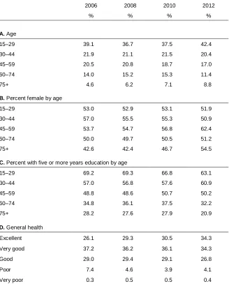
slight increase in the proportion of listed individuals living within the same compound as the primary respondent and the commensurate decrease in the proportion living in the same household (Panel F). Percent female (Panel B), percent with 5+ years of education (Panel C), general health (Panel D), and method of matching (Panel H) show fairly small fluctuations across waves.
Figure A-1: Study locations in Malawi
Table A-2 presents the match rates of individuals listed on the household rosters of
the analysis sample by selected characteristics in 2006‒2012. For the 2006‒2010
have affected sample characteristics (Table A-1). Match rates were similar in all age groups, although rates for the 60+ population in the 2006 wave lag behind the other waves somewhat. However, these ages are outside the prime ages where we would expect the effect of ART, and thus a differential in match rates is unlikely to bias our estimates. Match rates were generally higher for individuals who are closely related to the primary respondent (Panel B) and living geographically closer to the primary respondent (Panel C). Rates are comparable by sex (Panel D) and health status (Panel E). Overall, it does not appear that any systematic biases arise during the matching process, and the small variations in match rate that are observed occur in age ranges that are unlikely to affect our primary outcomes. Our findings on the increase in adult life expectancy post-ART are also robust to a number of alternative sample parameterizations (Table A-4).
Table A-1: Selected characteristics of the analysis sample
2006 2008 2010 2012
% % % %
A.Age
15‒29 39.1 36.7 37.5 42.4
30‒44 21.9 21.1 21.5 20.4
45‒59 20.5 20.8 18.7 17.0
60‒74 14.0 15.2 15.3 11.4
75+ 4.6 6.2 7.1 8.8
B.Percent female by age
15‒29 53.0 52.9 53.1 51.9
30‒44 57.0 55.5 55.3 50.9
45‒59 53.7 54.7 56.8 62.4
60‒74 50.0 49.7 50.5 51.2
75+ 42.6 42.4 46.7 54.5
C.Percent with five or more years education by age
15‒29 69.2 69.3 66.8 63.1
30‒44 57.0 56.8 57.6 60.9
45‒59 48.8 48.6 50.7 50.2
60‒74 34.8 36.1 37.5 32.2
75+ 28.2 27.6 27.9 20.9
D.General health
Excellent 26.1 29.3 30.5 34.3
Very good 37.2 36.2 36.1 34.3
Good 29.0 29.4 29.1 26.8
Poor 7.4 4.6 3.9 4.1
Table A-1: (Continued)
2006 2008 2010 2012
% % % %
E.Percent in poor/very poor health by age
15‒29 3.3 3.3 3.1 2.3
30‒44 5.5 5.7 5.1 5.5
45‒59 10.2 10.4 9.2 6.8
60‒74 22.7 18.7 17.8 20.2
75+ 35.9 35.9 31.2 41.8
F.Relationship to primary respondent
Respondent 24.4 20.5 19.7 14.4
Spouse 17.5 16.4 15.2 10.2
Child/child-in-law 26.8 29.2 36.2 62.8
Parent/parent-in-law 29.1 32.4 27.8 11.4
Other 2.2 1.5 1.1 1.2
G.Where individual usually lives
Same HH 55.6 46.1 44.4 37.8
Same compound 13.2 14.7 14.9 18.2
Same village 5.1 6.2 7.3 5.1
Same TA 9.7 12.5 13.1 13.6
Same district 7.6 7.5 8.6 8.7
Table A-1: (Continued)
2006 2008 2010 2012
% % % %
H.How individual matched
First round 98.8 97.8 98.7 99.1
Second round 0.3 1.1 0.3 0.3
Hand matched 0.9 1.1 1.0 0.6
N observations 7,481 8,883 7,913 3,733
N primary respondents 1,822 1,821 1,557 526
Table A-2: Match rate for analysis sample by selected characteristics
2006 2008 2010 2012
% % % %
Overall match rate 75.9 80.9 82.2 92.5
A.Age
15‒29 75.6 79.9 84.6 92.9
30‒44 83.1 85.6 89.0 97.3
45‒59 78.1 81.5 79.0 91.9
60‒74 67.9 80.1 74.4 89.3
75+ 62.4 77.4 75.8 85.0
B.Relationship to respondent
Respondent 96.9 98.0 98.0 97.7
Spouse 85.0 85.6 83.8 81.3
Child/child-in-law 77.5 83.5 92.1 96.1
Parent/parent-in-law 66.8 75.8 69.9 86.0
Table A-2: (Continued)
2006 2008 2010 2012
% % % %
C.Where individual usually lives
Same household 84.3 85.6 86.0 90.1
Same compound 70.1 79.9 83.3 95.4
Same village 65.1 78.4 76.0 93.2
Same traditional authority 69.4 73.8 75.7 93.4
Same district 65.0 80.0 80.9 95.0
Lilongwe 60.6 78.1 83.3 92.4
Blantyre 74.2 71.8 90.0 91.7
Elsewhere 64.7 74.7 77.5 92.8
D.Sex
Male 75.2 80.3 80.1 90.5
Female 76.5 81.4 84.2 94.5
E.General health
Excellent 80.3 80.7 84.4 93.4
Very good 76.9 82.5 82.4 92.4
Good 73.1 79.9 80.1 92.4
Poor 71.2 81.6 83.0 92.1
Table A-3: Adult life expectancy and median length of life by sex
A.Adult life expectancy
Period Years 95% CI
Male
2006‒2008 40.3 36.4 44.1
2008‒2010 43.0 39.6 46.5
2010‒2012 45.2 40.7 49.7
Post-ART (2008‒2012) 43.7 40.9 46.4
Female
2006‒2008 47.2 43.6 50.9
2008‒2010 47.0 43.4 50.5
2010‒2012 47.6 41.9 53.3
Post-ART (2008‒2012) 48.2 45.2 51.1
B.Median length of life
Period Years 95% CI
Male
2006‒2008 39 34 45
2008‒2010 45 41 49
2010‒2012 49 40 53
Post-ART (2008‒2012) 45 42 49
Female
2006‒2008 48 42 55
2008‒2010 50 44 56
2010‒2012 55 45 58
Post-ART (2008‒2012) 50 46 56
Table A-4: Adult life expectancy and median length of life for alternative definitions of the study population
Years 95% CI
A. Coresident with primary respondent
Adult life expectancy
2006‒2008 42.3 38.7 45.9
2008‒2010 44.8 41.5 48.1
2010‒2012 47.7 41.3 54.1
Post 46.6 43.7 49.4
Median age at death
2006‒2008 58 51 65
2008‒2010 67 59 69
2010‒2012 68 58 74
Post 67 64 70
B. All available observations
Adult life expectancy
2006‒2008 42.7 40.7 44.7
2008‒2010 43.4 41.7 45.2
2010‒2012 45.2 43.0 47.5
Post 44.1 42.7 45.5
Median age at death
2006‒2008 58 55 62
2008‒2010 60 59 62
2010‒2012 65 60 68
Table A-4: (Continued)
Years 95% CI
C. Matched in first round of matching
Adult life expectancy
2006‒2008 45.3 42.6 48.0
2008‒2010 48.2 45.6 50.8
2010‒2012 47.5 43.6 51.3
Post 47.9 45.7 50.0
Median age at death
2006‒2008 60 55 65
2008‒2010 66 62 69
2010‒2012 68 63 73
Post 67 64 69
D. Respondent, spouse, children, and parents only
Adult life expectancy
2006‒2008 43.0 40.4 45.6
2008‒2010 45.2 42.7 47.6
2010‒2012 45.9 42.2 49.5
Post 45.1 43.1 47.1
Median age at death
2006‒2008 58 54 63
2008‒2010 62 59 66
2010‒2012 67 60 70
Post 64 60 67