Effects of land use at a landscape scale on bumblebee nest density and survival

(1)

Patron: Her Majesty The Queen Rothamsted Research Harpenden, Herts, AL5 2JQ

Telephone: +44 (0)1582 763133 Web: http://www.rothamsted.ac.uk/

Rothamsted Research is a Company Limited by Guarantee Registered Office: as above. Registered in England No. 2393175. Registered Charity No. 802038. VAT No. 197 4201 51. Founded in 1843 by John Bennet Lawes.

Rothamsted Repository Download

A - Papers appearing in refereed journals

Goulson, D., Lepais, O., O'connor, S., Osborne, J. L., Sanderson, R. A.,

Cussans, J., Goffe, L. and Darvill, B. 2010. Effects of land use at a

landscape scale on bumblebee nest density and survival. Journal of

Applied Ecology. 47 (6), pp. 1207-1215.

The publisher's version can be accessed at:

• https://dx.doi.org/10.1111/j.1365-2664.2010.01872.x

The output can be accessed at:

https://repository.rothamsted.ac.uk/item/8q763

.

© Please contact library@rothamsted.ac.uk for copyright queries.

(2)

Effects of land use at a landscape scale on bumblebee

nest density and survival

Dave Goulson

1

*, Olivier Lepais

1

, Stephanie O’Connor

1

, Juliet L. Osborne

2

,

Roy A. Sanderson

3

, John Cussans

2

, Louis Goffe

3

and Ben Darvill

1

School of Biological & Environmental Sciences, University of Stirling, Stirling, FK9 4LA, UK;2Department of Plant & Invertebrate Ecology, Rothamsted Research, Harpenden, Hertfordshire, AL5 2JQ, UK; and3_{Institute for Research on} Environment and Sustainability, Devonshire Building, University of Newcastle, Newcastle-upon-Tyne, NE1 7RU, UK

Summary

1. We have little idea how landscape-scale factors inﬂuence the success of wild bumblebee nests over time. Here for the ﬁrst time we use molecular markers to estimate within-season changes in the numbers of nests.

2. Workers of two bumblebee species were sampled in an arable landscape in late May–June and late July–August, and the numbers of nests represented in each sample were estimated. We compare the methods available to estimate nest number from such samples and conclude that methods which allow for heterogeneity in the probability of capture of nests provide the best ﬁt to our data. Changes in numbers of nests at the two time points were used to infer nest survival.

3. The two bee species appeared to differ markedly in survival over time, with estimates of 45% of nests surviving forBombus lapidariusand 91% forB. pascuorum. However, our data suggest that the foraging range ofB. pascuorummay be greater in late season, which would lead us to overesti-mate nest survival in this species. Differential survival may also reflect differences in phenology between the two species.

4. The land use class which had the most consistent effects on nest number and survival was gar-dens; forB. lapidarius, the area of gardens within a 750 and 1000 m radius positively influenced nest survival, while forB. pascuorum, the number of nests in late samples was higher at sites with more gardens within a 500 and 750-m radius. ForB. pascuorum, the area of grassland within a 250 and 500-m radius also positively influenced nest number in late samples, probably because this is the pre-ferred nesting habitat for this species.

5. The importance of gardens is in accordance with previous studies which suggest that they now provide a stronghold for bumblebees in an otherwise impoverished agricultural environment; fur-thermore, our data suggest that the positive inﬂuence of gardens on bumblebee populations can spill over at least 1 km into surrounding farmland.

6. Synthesis and applications.The substantial eﬀects that even small areas of local resources such as rough grassland or clover leys can have on bumblebee nest numbers and survival is of clear relevance for the design of pollinator management strategies.

Key-words: Bombus, density, gardens, kinship, microsatellite, mortality, pollination services, population structure, social insects

Introduction

There is mounting evidence that bumblebees and other key pollinators have declined in Western Europe, North America, and parts of Asia (Goulson, Lye & Darvill 2008; Brown &

Paxton 2009; Williams & Osborne 2009). These declines raise concerns about the provision of pollination services for both crops and wildﬂowers, and there is growing interest in manag-ing the landscape to combine anthropogenic needs with provi-sion of ecosystem services such as pollination (e.g. Isaacset al.

2009; Lonsdorfet al.2009).

(3)

(notably in bumblebees). Studies which have manipulated hab-itats to examine the effect on pollinators tend to focus on counts of workers (e.g. Kells, Holland & Goulson 2001; Carvellet al.2007; Heardet al.2007), but ideally we would like to know how these manipulations impact on nest density and survival. One approach by which it is possible to indirectly measure nest number is via DNA sampling of workers. If workers are typed at sufficient microsatellite loci, it is possible to identify groups of sisters each representing a nest. These data can then be further analysed to estimate how many nests were foraging at a site but by chance were not represented in the sampled bees; the approach used for this has been to fit the data to a Poisson distribution. This method has previously been used to quantify the numbers of nests visiting particular flower patches (Chapman, Wang & Bourke 2003), to quantify foraging range by examining the distribution of sisters along a transect (Darvill, Knight & Goulson 2004; Knightet al.2005) and to estimate population size in isolated populations of a rare bumblebee (Elliset al.2006). These studies have provided valuable insights into aspects of bumblebee ecology that had previously proved to be intractable.

For social insects such as bumblebees to thrive, they require suitable forage throughout the period of colony development (spring and summer). Modern agricultural landscapes consist of large areas of monocultures separated by ﬁeld margins and interspersed by occasional patches of non-cropped areas (e.g. woodland) and clusters of housing with gardens (Osborne

et al.2008a). Some crop monocultures such as oilseed rape and field beans provide massive but short-lived bursts of floral resources during the season. This spatial and temporal patchi-ness of floral resources is likely to mean that bumblebee nests fare differently depending on where they are located in the agri-cultural landscape. However, because of the difficulty in find-ing bumblebee nests, we have very little information on nest survival rates and how nest density changes through the sea-son.

Here, we study changes in nest density over time in two bumblebee species,B. pascuorum andB. lapidarius. We use DNA sampling of workers to detect sisters and infer nest num-ber early in the season (late May–June) and late in the season (late July–August). We compare different approaches to esti-mating the numbers of nests present using such genetic sam-ples. Our estimates of nest density in early and late season, and of nest survivorship, are examined in relation to a detailed remote-sensed land use map of the study area. This enables us to examine which land use classes influence nest density and survival, and over what spatial scale these effects are detected on the two contrasting bee species. Our results have clear impli-cations for the management of pollination services in arable landscapes.

Materials and methods

S A M P L E C O L L E C T I O N

The study was carried out in a 10·20 km rectangle centred on Rothamsted Research (Harpenden, Hertfordshire, UK) where

several studies of bumblebee foraging range and population size have already been conducted (Knightet al. 2005, 2009; Osborneet al.

2008a). Samples ofB. lapidariusandB. pascuorumworkers were col-lected from along a 200·10 m strip of a ﬁeld margin at each sample site. Worker bees were sampled at the same sites on two occasions in 2007: between the 22 May and the 22 June (= early samples) and between the 25 July and 9 August (= late samples). Each site was vis-ited repeatedly during each sample period until at least 50 bees of each species had been sampled or until the sampling period ended. Four-teen sites were selected for sampling, on the basis that they were at least 1 km apart and 1 km from any substantial urban area (Fig. S1, Supporting Information).

A total of 1660B. pascuorumworkers and 1083B. lapidarius work-ers were caught (Tables 2 and 3). A non-lethal tarsal sample from a mid-leg (Holehouse, Hammond & Bourke 2003) was taken from each worker during the early sample, and foraging workers were collected during the late sample. All samples were preserved in ethanol.

M O L E C U L A R M E T H O D S

DNA was extracted using the HotShot protocol (Holehouse, Ham-mond & Bourke 2003).B. lapidariusindividuals were genotyped at ten microsatellites (BL11, BL06, BT24, BT09, BT18, B126, B96, B10, B11 and B118) andB. pascuorumindividuals at nine microsatellites (BL03, BT10, BT26, BT18, B124, B126, B96, B132 and B118) (Estoup

et al.1995; Funk, Schmid-Hempel & Schmid-Hempel 2006). Micro-satellite loci were ampliﬁed with a multiplex protocol following Darv-illet al.(2006) and described in detail elsewhere (Lepaiset al.2010). The genetic data are archived in the Dryad database (available at http://hdl.handle.net/10255/dryad.1113).

L A N D S C A P E C H A R A C T E R I Z A T I O N

A detailed composition of the landscape around each sample site was created. The process consisted of identifying the key land cover clas-ses and utilizing remote sensed data, digital cartography or a combi-nation of the two to identify the feature in the study area. The two input datasets used for the generation of the land cover classification were IKONOS satellite imagery (4 m multispectral and 1 m panchro-matic) and Ordnance Survey MasterMap topographic layer. These were processed using a combination of remote sensing and GIS tech-niques using ERDAS IMAGINE 9Æ1 and ESRI ArcGIS desktop 9Æ2. The incorporation of MasterMap (vector) data into the procedure means that the boundaries of specific features could be accurately defined (Fig. S1). Where classes were found to overlap, priority in the final classified map was given according to physical structure, e.g. trees were given priority over grass. Table S1 in Supporting Informa-tion provides a summary of each land cover class plus the dataset from which it was derived.

S T A T I S T I C A L M E T H O D S

Genetic comparison of early and late samples

We used the complete dataset, i.e., all workers regardless of the sib-ship reconstruction, including sites that had at least 10 sampled work-ers and excluding the outlier site E (see ‘Results’ section covering sibship reconstruction) to compare genetic parameters between early and late samples. We usedfstatversion 2.9.3.2 (Goudet 1995) to

com-pute allelic richness obtained by rarefaction (Petit, El Mousadik & Pons 1998), observed heterozygosity, gene diversity (Nei 1987), heterozygosity deﬁcit, population diﬀerentiation (Weir & Cockerham

1208 D. Goulsonet al.

(4)

1984) and average relatedness within groups (Queller & Goodnight 1989). We compared these parameters between early and late samples. The signiﬁcance of each comparison was tested using 1000 permutations of individuals between samples. TheP-value of the test was computed as the proportion of randomized data sets giving a larger parameter than that calculated from the observed data sets.

Sibship reconstruction

We used the maximum likelihood sibship reconstruction method implemented incolonysoftware version 1.2 (Wang 2004) to identify

workers that belonged to the same colony. This software was found to produce the most accurate sibship reconstruction, in particular in the presence of genotyping error (Lepaiset al.2010). We ran the soft-ware with the following options: haplo-diploid species; sex 1 set as diploid females; allele frequencies updated each 1000 iterations; 2% genotyping error for all loci (0Æ5% of allele dropout and 1Æ5% other errors).

Nest number and survival estimations

Truncated Poisson method. Based on the sibship reconstruction obtained from COLONY, we counted the number of nests repre-sented by 1, 2, 3,…,kworkers. We estimated the number of unsam-pled nests by ﬁtting a truncated Poisson distribution to the data and extrapolating this distribution to the zero class, an approach previ-ously used on similar data sets (Chapman, Wang & Bourke 2003; Darvill, Knight & Goulson 2004; Knightet al.2005). This statistical method assumes that there is an equal probability of sampling work-ers from all of the nests which forage at the site. In practice, due to heterogeneity in nest size and location, it is probable that some nests are more likely to be sampled than others.

Applying DNA mark–recapture methods. Recent developments in the ﬁeld of DNA-based capture–recapture models allow for multiple sampling of an individual. The number of times an individual is recaptured can be used to estimate the population size (Miller, Joyce & Waits 2005). This method is often used on data obtained from non-invasive DNA sampling, such as number of scats or hairs sampled per individual. Our data are similar, albeit that instead of trying to estimate the number of individuals we are interested in estimating the number of nests represented in our sample of workers. Interestingly, Capwire software (Miller, Joyce & Waits 2005) implements two meth-ods. The Event Capture Model (ECM) assumes that each individual has an equal probability of being sampled, an assumption similar to the truncated Poisson methods described above. The Two Innate Rate Model (TIRM) allows for heterogeneity in capture probability

among individuals. Furthermore, Capwire uses a likelihood ratio test to find the best model to estimate the population size. We used this likelihood ratio test to find out which model would give the better fit to our data and subsequently used both ECM and TIRM models to estimate the number of nests foraging at each sample site. We finally compared these estimations with the previously used truncated Pois-son method.

The values for nest numbers estimated by Capwire software (using the TIRM model) were used in subsequent analyses. Nest detectabil-ity was calculated as the ratio of detected nests to the total number of nests estimated to be present at each time point. This is simplistic since it makes the assumption that capture probability is equal for all nests. However, it enables us to estimate nest survival across the two sample time points, taking into account changes in detectability (see Table 2).

Impact of surrounding land use on nest number and survival

We chose to consider all land cover types as predictor variables in order to avoid potential issues associated with biased variable selec-tion (Whittinghamet al. 2006). We used hierarchical partitioning (HP) (Chevan & Sutherland 1991) to estimate for each predictor vari-able its independent and conjoint contribution with all other varivari-ables in a multiple linear regression setting, using the hier.part package (MacNally & Walsh 2004) of the R software (R Development Core Team 2005). Generalized linear models were run using a Poisson dis-tribution (for count data) for performing the analysis of nest number in early and late samples, and with a Gaussian distribution when nest survival was the response variable. To identify the most important predictor variables, the randomization procedure was used (1000 ran-domizations performed) to test the signiﬁcance of the independent contribution of each predictor (MacNally 2002). We performed the analysis independently for each landscape radius (250, 500, 750 and 1000 m) and each species, excluding the outlier site E.

Results

C O M P A R I S O N O F P O P U L A T I O N G E N E T I C P A R A M E T E R S B E T W E E N S A M P L I N G P E R I O D S

Most of the population genetic parameters showed a signiﬁ-cant diﬀerence between early and late samples inB. lapidarius

(Table 1). Genetic diversity (RsandHs) signiﬁcantly decreased, probably due to a higher family structure in late samples (lower numbers of nests and higher numbers of workers from

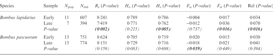
Table 1.Comparison of genetic parameters among sites and sampling periods

Species Sample Npop Nind Rs(P-value) Ho(P-value) Hs(P-value) Fis(P-value) Fst(P-value) Rel (P-value)

Bombus lapidarius Early 11 607 8Æ241 0Æ789 0Æ786 )0Æ004 0Æ017 0Æ034

Late 7 394 7Æ419 0Æ771 0Æ762 )0Æ012 0Æ036 0Æ070

P-value (0Æ002) (0Æ215) (0Æ005) (0Æ737) (0Æ016) (0Æ016)

Bombus pascuorum Early 13 751 8Æ624 0Æ705 0Æ719 0Æ020 0Æ015 0Æ030

Late 13 774 8Æ151 0Æ729 0Æ716 )0Æ018 0Æ021 0Æ041

P-value (0Æ159) (0Æ083) (0Æ698) (0Æ039) (0Æ449) (0Æ394)

Npop: number of sites,Nind: number of individuals,Rs: allelic richness (Petit, El Mousadik & Pons 1998) rareﬁed to 21 and 49 individuals

forB. lapidariusandB. pascuorum, respectively,Ho: observed heterozygosity andHs: gene diversity (Nei 1987),Fis: heterozygosity deﬁcit

andFst: genetic diﬀerentiation (Weir & Cockerham 1984), Rel: average relatedness (Queller & Goodnight 1989).P-values are obtained

(5)

common nests) as shown by the significant increase in genetic relatedness (Rel) and genetic differentiation (Fst). Although the same trends are observed in B. pascuorum, the differences between early and late samples were smaller and were not sig-nificant (Table 1), with the exception of the deficit of hetero-zygotes (Fis) which was lower for late samples.

N E S T N U M B E R E S T I M A T I O N S

We found that the Even Capture Model (ECM) gave very simi-lar estimates of the total number of nests present in a site com-pared to the truncated Poisson method (Fig. 1). However, using the likelihood ratio test (LRT), the Two Innate Rates Model (TIRM) was the more likely model in 18 out of 22 sam-ples (82%) forB. lapidariusand 21 out of 28 samples (75%) for

B. pascuorum. Simulated data using a range of degrees of heter-ogeneity in capture probability showed that the LRT rejected the ECM model in favour of the correct TIRM model only in about 30% of the cases (Miller, Joyce & Waits 2005). Given that a high percentage of selected TIRM models were selected to ﬁt our data (82% and 75%), it appears that heterogeneity of capture probability is a strong characteristic of the nests. Thus the Capwire’s TIRM model probably gave more accurate esti-mates of the number of nests foraging at a site. These estiesti-mates were approximately 1Æ4 times higher than the estimations pro-duced using the Poisson method (Fig. 1). For subsequent anal-yses of the eﬀects of landscape variables on nest numbers and survival we therefore used nest number estimates produced using the TIRM method (Tables 2 and 3).

The estimates for the total number of nests forB. lapidarius

ranged from 32 to 416 in early samples and from 15 to 127 in late samples (Table 2). Site E appeared to contain many more nests than other sites (excluding site E, nest number ranged

from 32 to 215 in early samples and from 15 to 45 in late sam-ples). Estimated nest survival ranged from 0Æ25 to 0Æ87 (Table 2). The estimate of the total number of nest for

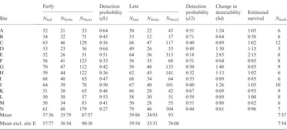
B. pascuorumranged from 33 to 179 in early samples and from 17 to 313 in late samples (Table 3). Again, site E appeared to be an outlier. Nest survival ranged from 0Æ38 to 2Æ15 including all sites or from 0Æ38 to 1Æ13 excluding site E (Table 3).

Site E was highly atypical for both bee species; these results are likely to be explained by the presence of a 5-ha clover ley in close proximity to the sample area, a land cover type that is rare in the study area. Hence we chose to exclude site E from all subsequent analyses.

Estimated survival varied signiﬁcantly between species (pairedt-test,t7= 6Æ05,P= 0Æ001), being consistently lower at all sites forB. lapidariusthan forB. pascuorum(Tables 2 and 3).

Some nests were detected in both early and late samples. It is informative to compare this number to the number of nests which we would expect to observe in both samples. ForB. lapi-darius, we directly observed 414 nests across all sites in the first sample, but estimated that in total there were 1372 nests pres-ent. The proportion of ‘marked’ nests (i.e. those sampled and genotyped) was therefore 0Æ301. So long as detected nests were not more or less likely to die than undetected nests (unlikely, as we used non-lethal tarsal sampling), in the second sample in which we directly detected 206 nests, we would expect 62 of these to be nests also directly detected in the first sample. The actual figure for the number of nests detected in both samples is 80 (Fisher’s exact test, two-tailed,P= 0Æ078).

ForB. pascuorum, we directly observed 501 nests in the ﬁrst sample, and estimated that 1226 nests were foraging at sample sites (i.e. the proportion directly detected was 0Æ409). Of the 489 nests directly detected in the second sample, we would expect 200 to have been previously detected in the ﬁrst sample, but in fact only 106 nests were detected in both samples (Fish-er’s exact test, two-tailed,P< 0Æ001).

I M P A C T O F S U R R O U N D I N G L A N D U S E O N N E S T N U M B E R A N D S U R V I V A L

For B. lapidarius, the HP analysis showed that the area of woodland within a radius of 1000 m had a positive impact on the number of nests visiting the site in the early sample, while the area of woodland within 250 m had a negative impact on the number of nests in late samples (Fig. 2; Fig. S2, Support-ing Information). Nest survival was signiﬁcantly and positively associated with the area of gardens within both 750 and 1000 m (Fig. 2). This occurred despite the deliberate selection of sample sites away from urban areas; the highest proportion of gardens within 1000 m of any site was 5Æ1%. Nest survival was negatively predicted by the area of woodland within 500 m.

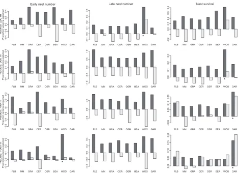
ForB. pascuorum, the area of woodland within a radius of 750 and 1000 m and the area of made-made surface within a radius of 1000 m had a positive impact on early nest number, while the number of nests in late samples was positively associ-ated with the area of grassland within radii of 250 and 500 m 0 50 100 150 200 250

0

5

0

100

150

200

250

Truncated Poisson – number of nests

Capwire − n

umber of nests

Capwire − ECM Capwire − TIRM

Fig. 1.Comparison of estimated total nest number for the two species combined by the extrapolation of a truncated Poisson distribution and DNA mark–recapture method (Capwire) implementing the even capture model (ECM) and the two innate rates model (heterogeneity of capture probability; TIRM). Dashed line indicates equality of esti-mation between models (regression slope of 1).

(6)

and also with the area of gardens within 500 and 750 m (Fig. 3). The area of man-made land cover within a radius of 750 m was found to be positively correlated with nest survival (Fig. 3).

Discussion

Previous studies using microsatellite data to estimate colony number from samples of worker bumblebees have assumed

that the number of nests detected by one, two, three, etc. work-ers follow a Poisson distribution, allowing estimation of the number of nests not detected (the zero category) (Chapman, Wang & Bourke 2003; Darvill, Knight & Goulson 2004; Knight et al. 2005, 2009; Ellis et al. 2006). These studies acknowledged that this approach is probably inaccurate since it assumes that all nests are equally likely to be sampled, an assumption which is clearly not valid (nests are likely to vary both in size and in their distance from the sample site). Here we Table 2.Nest number estimations forBombus lapidarius

Site

Early Detection

probability (d1)

Late Detection

probability (d2)

Change in detectability (dd)

Estimated survival Nboth

NInd NNobs NNtot1 NInd NNobs NNtot2

A 27 23 100 0Æ23 0 – – – – – –

B 38 21 46 0Æ46 4 3 – – – – –

C 68 36 75 0Æ48 60 17 20 0Æ85 0Æ56 0Æ47 11

D 34 22 49 0Æ45 5 5 - - – – –

E 50 47 416 0Æ11 55 41 127 0Æ32 0Æ35 0Æ87 9

F 53 34 83 0Æ41 50 23 42 0Æ55 0Æ75 0Æ68 7

G 68 36 73 0Æ49 55 27 45 0Æ60 0Æ82 0Æ75 12

H 81 60 178 0Æ34 51 25 42 0Æ60 0Æ57 0Æ42 10

I 48 21 32 0Æ66 7 6 21 0Æ29 2Æ30 0Æ29 9

J 3 2 – – 50 14 15 0Æ93 – – 1

K 71 30 54 0Æ56 21 9 17 0Æ53 1Æ05 0Æ30 7

L 49 24 51 0Æ47 7 6 21 0Æ29 1Æ65 0Æ25 4

M 2 2 – – 5 4 – – – – –

N 70 56 215 0Æ26 52 26 43 0Æ60 0Æ43 0Æ46 10

Mean 47Æ29 29Æ57 114Æ33 30Æ14 15Æ85 39Æ3 8Æ00

Mean excl. site E 47Æ08 28Æ23 86Æ91 28Æ23 13Æ75 29Æ56 7Æ89

NInd: number of sampled workers at each time point,NNobs: number of observed nests (based on Colony fullshib reconstruction),NNtot:

total nest number including the unsampled nests (based on Capwire TIRM model estimations). Detection probabilities (d) are the pro-portion of detected nests relative to the total estimated number of nests. The change in detectability (dd) isd1⁄d2. Estimated survival, taking into account changes in detectability, is given by (Ntot2⁄dd)⁄Ntot1.Nboth= no. of nests detected in both early and late samples.

Table 3.Nest number estimations forB. pascuorum

Site

Early Detection

probability (d1)

Late Detection

probability (d2)

Change in detectability (dd)

Estimated survival Nboth

NInd NNobs NNtot1 NInd NNobs NNtot2

A 52 21 33 0Æ64 50 22 43 0Æ51 1Æ24 1Æ05 6

B 54 32 71 0Æ45 53 12 17 0Æ71 0Æ64 0Æ38 6

C 63 46 129 0Æ36 66 47 117 0Æ40 0Æ89 1Æ02 12

D 53 23 36 0Æ64 49 26 53 0Æ49 1Æ30 1Æ13 5

E 52 26 51 0Æ51 64 56 313 0Æ18 2Æ85 2Æ15 8

F 56 41 125 0Æ33 56 35 68 0Æ51 0Æ64 0Æ85 8

G 70 47 112 0Æ42 50 40 133 0Æ30 1Æ40 0Æ85 9

H 59 44 122 0Æ36 62 45 141 0Æ32 1Æ13 1Æ02 6

I 68 40 85 0Æ47 68 34 64 0Æ53 0Æ89 0Æ85 6

J 64 39 78 0Æ50 67 40 101 0Æ40 1Æ26 1Æ03 10

K 51 30 65 0Æ46 66 28 42 0Æ67 0Æ69 0Æ93 9

L 50 30 57 0Æ53 58 30 51 0Æ59 0Æ89 1Æ00 8

M 50 34 83 0Æ41 50 28 55 0Æ51 0Æ80 0Æ82 6

N 61 48 179 0Æ27 79 46 104 0Æ44 0Æ61 0Æ96 7

Mean 57Æ36 35Æ79 87Æ57 59Æ86 34Æ93 93 7Æ57

Mean excl. site E 57Æ77 36Æ54 90Æ38 59Æ54 33Æ31 76Æ08 7Æ54

NInd: number of sampled workers at each time point,NNobs: number of observed nests (based on Colony fullshib reconstruction),NNtot:

(7)

explore the use of the program Capwire (Miller, Joyce & Waits 2005) to estimate the number of nests present. This software allows us to either assume that nests have an equal probability of capture (the Event Capture Model, ECM), or that the prob-ability of capture varies (the Two Innate Rate Model, TIRM). We demonstrate that the former gives estimates of nest number that are nearly identical to those obtained from the use of a Poisson distribution. Likelihood ratio tests implemented in Capwire suggested that the TIRM provides a better ﬁt to our data for both bee species. The TIRM method produced esti-mates of the number of nests present which were consistently higher by around 40%. It therefore seems likely that the nest density and colony number estimates derived in previous stud-ies were underestimates.

The main purpose of our study was to derive estimates of nest number from multiple sites and at two points in time (late May–June and late July–August), and to use these data to examine how the surrounding land use influenced changes in nest number over time. There have been very few previous esti-mates of bumblebee nest survivorship, reflecting the difficulty in finding sufficient nests to obtain meaningful data. Our data allow us to indirectly estimate survivorship over an approxi-mately 2-month period which roughly corresponds to the last 2 months of nest development.

Our estimates must be interpreted with care. We can account for changes in detection probability over time, which we might expect as nests grow larger. However, the number of nests detected at each time point will also be inﬂuenced by any sea-sonal changes in foraging range. Although there was noa pri-orireason to believe that foraging ranges systematically change through the season, our data provide evidence that they do in

B. pascuorum.

ForB. lapidarius, in the early sample, we directly detected 414 nests, and estimate that there were another 958 that we had not caught, so that we have recognizable genotypes for 30% of the population. In the second sample we directly detected 206 nests of which 80 (37%) were also in the ﬁrst sam-ple. If foraging range remained unchanged, we would expect the proportion to remain unchanged, regardless of mortality. In this instance the proportion is similar, suggesting that forag-ing range has indeed not changed substantially. We would not see this pattern if, for example, high nest mortality was being oﬀset by increasing foraging range (this would give us an apparently high nest survivorship but an unexpectedly low recapture rate).

In contrast, forB. pascuorum, we directly detected 501 nests in the ﬁrst sample, and estimate that there were a further 725 that we did not detect, so that we have recognizable genotypes

FLB MM GRA CER OSR BEA WOO GAR

Propor tion v a ri ance e xplained −0·1 0·0 0 ·1 0·2 0 ·3 *

−0·4 −0·2 0·0 0 ·2 0·4

0·00 0·05 0·10 0·15 0·20 * Radius: 1000 m

Propor tion v a ri ance e xplained −0·2 −0·1 0·0 0 ·1 0·2 0 ·3

−0·5

0·0

0

·5

−0·05 0 ·05 0 ·10 0 ·15 * Radius: 750 m

Propor tion v a riance e xplained −0·1 0·1 0·2 0·3 0·4

−1·0

−0·5

0·0

0·5

1·0

0·0 0·1 0·2 0·3 * Radius: 500 m

Propor tion v a riance e xplained −0·4 −0·2 0·0 0·2 0·4

−0·1 0·0 0·1 0·2 0·3 0·4 *

−0·2 0·0 0·1 0·2 0·3 0·4

Early nest number Late nest number Nest survival

Radius:

250 m

Fig. 2.Hierarchical partitioning showing independent (black) and conjoint (grey) effects of landscape variables expressed as the percentage of the total variance explained forBombus lapidarius. FBL, field boundary length; GRA, grass; OSR, oilseed rape; WOO, wood; MM, man made; CER, cereal; BEA, bean; GAR, garden. *Significant independent contribution of a predictor variable at a 0Æ05 level.

(8)

for 41% of the population. In the second sample we directly detected 489 nests of which 106 (21%) were also in the first sample, a significant decrease. The numbers of nests detected at each time point suggest little mortality, but the unexpectedly low number of recaptures (21% compared to 41%) strongly suggests that we are sampling from a larger pool on the second occasion, which (given that nests are fixed and that there is no reproduction) can only be explained by increasing foraging range.

Our data suggest marked differences in the survival of the two species, withB. lapidariushaving a mean survival rate of 0Æ45 over this2 month period compared to 0Æ94 inB. pascuo-rum. However, our estimates of survival taking into account nest detectability make the assumption of equal detection probability for all nests, something which our own analyses of methods for estimating the number on non-detected nests sug-gest is untrue. If workers ofB. pascuorumare foraging further afield during the late sample period then we might expect this to increase heterogeneity in detectability among nests, inflating estimates of nest numbers at this time and therefore inflating estimates of nest survival. Conversely, there is some evidence that B. lapidarius may have suffered greater mortality than

B. pascuorum. B. lapidarius has a southerly distribution compared toB. pascuorum, and 2007 was an exceptionally cool

and wet summer, so we might have expectedB. lapidariusto fare poorly. The low abundance ofB. lapidarius relative to

B. pascuorum in this year is reflected in the sample sizes obtained for the two species; forB. pascuorumit was relatively easy to obtain the target figure of50 bees per site per sample period. In contrast, for B. lapidarius, sample sizes for two sample sites in the early period and six in the later period were too small to allow analysis (Table 2). An alternative explana-tion for differences in survival is that it is driven by phenology.

B. pascuorumnests can last through to September whileB. lapi-dariusnests tend to die oﬀ by late July⁄August, the time at which we took the second sample. This might explain why

B. lapidariusapparently exhibited higher nest mortality, for nests were approaching the end of their natural life.

The particular landscape factors that were found to affect nest number and survivorship differed between species, but one factor was consistent for both. The area of gardens within 750 or 1000 m was found to positively influence nest survivor-ship in B. lapidarius, while the area of gardens within 500 and 750 m was found to positively influence the number of

B. pascuorumnests in the late sample. Young nests ofB. terres-trisplaced in suburban gardens have been found to grow more quickly when compared to nests placed in arable farmland (Goulson et al.2002). Osborneet al. (2008b) used a public

Propor tion v a riance e x plained −0·1 0·0 0 ·1 0·2

0·0 0 ·1 0·2 0·3 *

−0·3

−0·1

0·1

0·3

Propor tion v a riance e xplained 0·00 0 ·05 0 ·10 0·15

−0·05 0·05 0·10 0·15 0·20 * *

−0·1 0·0 0·1 0·2 0·3 0 ·4

Propor tion v a ri ance e x plained −0·1 0 ·0 0·1 0 ·2 0·3 *

−0·10

0·00

0·10

0·20

*

−0·2 0 ·0 0·2 0 ·4 0·6 *

Propor tion v a ri ance e x plained −0·1 0 ·1 0·2 0 ·3 0·4 * *

−0·1 0 ·0 0·1 0 ·2 0·3

−0·2 0 ·0 0·2 0 ·4 0·6

Early nest number Late nest number Nest survival

Radius: 1000 m R adius: 750 m R adius: 500 m R adius: 250 m

(9)

survey to quantify bumblebee nest densities and found the highest nest densities in gardens. The present study was not specifically designed to examine the impacts of urban areas; the highest proportion of habitat classed as garden within 1 km of our study sites was 5Æ1%. Our data suggest that not only are gardens important for bumblebees even when they represent a small proportion of the landscape, but also that their positive influence on bumblebee populations can spill over onto neighbouring farmland that is 1 km distant. The positive relationships between the numbers of nests detected and the area of gardens nearby found for both bee species have two possible explanations. It may be that these nests are situ-ated in the farmland, but benefiting from the floral resources obtained from gardens, or it may be that these nests are situ-ated in gardens, in which case it may be that gardens are pro-viding both floral resources and nest sites. Under either scenario, our results suggest that lack of resources in farmland is currently limiting pollinator populations.

Aside from gardens, the only significant land use to influ-ence nest number ofB. lapidariuswas woodland; nest number in the early sample was higher at sites with more woodland within 1000 m, but nest number in the late sample period was lower at sites with more woodland within 250 m and nest sur-vival was negatively correlated with area of woodland within 500 m. We have only speculative explanations for these results. Woodland in this area is typically deciduous, and deciduous woodland provides plentiful spring flowers such as bluebells. However, once the tree canopy closes inMay there are few flowers. It may be that woodland spring flowers are important toB. lapidariusqueens, and so boost the number of nests found in the early sample period. Conversely, woodland later in the season may provide an obstacle to foragers, so that woodland close to nests is particularly disadvantageous.

The factors inﬂuencing nest numbers for B. pascuorum

(other than gardens) are more readily explained.B. pascuorum

numbers in early samples were positively associated with the area of woodland within 750 and 100 m, and in late samples with the area of grassland within 250 and 500 m.B. pascuorum

tends to nest above the ground in grass tussocks, leaﬂitter and thickets, so these land use categories are likely to be providing nest sites (Goulson 2003).

We found no significant effect of either oilseed rape or field beans on nest number at either time point, nor any effect on survival. Previous studies of the effects of mass-flowering crops on bumblebee populations have produced mixed results. Herr-mannet al.(2007) found no effect of mass-flowering crops on the number ofB. pascuorumnests detected using microsatellite markers. Westphal, Steffan-Dewenter & Tscharntke (2009) examined colony growth ofB. terrestris, and found greater colony growth in early season when artificial nests were placed near oilseed rape field, but they found no effect on colony reproduction. Perhaps the most marked contrast between our findings and previous work is with Knightet al.(2009), who studied the same area as ourselves in 2004 using an essentially similar approach. Knight et al.(2009) sampled bees in late July (hence equivalent to our late sample period). They found that the area of field beans, oilseed rape and non-cropped area

(including gardens) within 1 km of each sample site was posi-tively correlated with the number of B. pascuorum nests detected. Their landscape classiﬁcation was much simpler than ours; they did not have separate garden and grassland catego-ries, both of which were signiﬁcant predictors ofB. pascuorum

nest abundance in our late samples. These differences in meth-odology may explain the differences in results obtained, but it is also possible that the relative importance of different land-scape factors varies from year to year, according to the weather and bumblebee population density.

Our results have practical relevance for farmers wishing to maximize pollination services to their crops. Crops grown within 1 km of gardens are likely to receive more visits from bumblebees. Those growing deep-flowered crops such as field beans might consider ensuring that there are areas of rough grassland within 750 m of their bean fields to boost popula-tions of B. pascuorum. Although unreplicated and hence anecdotal, the marked difference between site E and our other sample sites illustrates that on-farm management can have a striking effect on bee numbers. This site appeared to have approximately four times as manyB. lapidariusnests in both early and late samples, and approximately five times as manyB. pascuorumin late samples, compared to other sites. These large differences are almost certainly attributable to a 5-ha clover ley adjacent to this site. Clover leys were once a common feature on arable farms since they boost soil fertil-ity, but the advent of cheap artificial fertilizers led to their abandonment; it has been argued that this change in farming may have played a significant role in driving bumblebee declines in the twentieth century (Goulsonet al.2005, 2008). It would appear that reinstatement of clover leys may pro-vide a swift way to rapidly boost bumblebee numbers on farmland (Carvellet al.2006, 2007).

Our study is one of the first to provide estimates of changes in nest density over time in bumblebees, and suggests that there may be differences between species in their patterns of seasonal mortality. Interpretation of our data is complicated by appar-ent changes in the foraging range of one of the two study spe-cies through the season. If, as suggested by the data, B. pascuorumare forced to forage further afield in late season due to a paucity of forage, then this would argue that conservation measures might better target forage provision in late July⁄ August rather than late May⁄June.

In addition to the diﬃculties posed by varying foraging range, our approach is clearly not suitable for examining the early stages of colony development when only the queen is present, or when workers are very scarce. This is unfortunate as many authors have speculated that this is likely to be the time when most nest mortality probably occurs (e.g. Goulson, Lye & Darvill 2008); a major challenge for future research is to develop means of examining survivorship in the early season, from queen emergence onwards.

Acknowledgements

We thank the farmers in Hertfordshire for allowing us to sample bees from their land, Niccolo` Alfano for help with sample collection, two anonymous reviewers

(10)

for comments and Michael Pocock for advice on the analyses. This project was

funded by the BBSRC; project number BB⁄E000932⁄1.

References

Brown, M.J.F. & Paxton, R.J. (2009) The conservation of bees: a global

per-spective.Apidologie,40, 410–416.

Carvell, C., Roy, D.B., Smart, S.M., Pywell, R.F., Preston, C.D. & Goulson, D. (2006) Declines in forage availability for bumblebees at a national scale.

Biological Conservation,132, 481–489.

Carvell, C., Meek, W.R., Pywell, R.F., Goulson, D. & Nowakowski, M. (2007) Comparing the eﬃcacy of agri-environment schemes to enhance bumblebee

abundance and diversity on arable farmland.Journal of Applied Ecology,44,

29–40.

Chapman, R.E., Wang, J. & Bourke, A.F.G. (2003) Genetic analysis of spatial

foraging patterns and resource sharing in bumble bee pollinators.Molecular

Ecology,12, 2801–2808.

Chevan, A. & Sutherland, M. (1991) Hierarchical partitioning.American

Stat-istician,45, 90–96.

Darvill, B., Knight, M.E. & Goulson, D. (2004) Use of genetic markers to

quantify bumblebee foraging range and nest density.Oikos,107, 471–478.

Darvill, B., Ellis, J.S., Lye, G.C. & Goulson, D. (2006) Population structure

and inbreeding in a rare and declining bumblebee, Bombus muscorum

(Hymenoptera: Apidae).Molecular Ecology,15, 601–611.

Ellis, J.S., Knight, M.E., Darvill, B. & Goulson, D. (2006) Extremely low eﬀec-tive population sizes, genetic structuring and reduced genetic diversity in a

threatened bumblebee species,Bombus sylvarum(Hymenoptera: Apidae).

Molecular Ecology,15, 4375–4386.

Estoup, A., Tailliez, C., Cornuet, J.M. & Solignac, M. (1995) Size homoplasy

and mutational processes of interrupted microsatellites in 2 Bee species,Apis

melliferaandBombus terrestris(Apidae).Molecular Biology and Evolution,

12, 1074–1084.

Funk, C.R., Schmid-Hempel, R. & Schmid-Hempel, P. (2006) Microsatellite

loci for Bombus spp.Molecular Ecology Notes,6, 83–86.

Goudet, J. (1995) FSTAT (Version 1.2): A computer program to calculate

F-statistics.Journal of Heredity,86, 485–486.

Goulson, D. (2003)Bumblebees; Their Behaviour and Ecology. Oxford

Univer-sity Press, Oxford.

Goulson, D., Lye, G.C. & Darvill, B. (2008) Decline and conservation of

bum-blebees.Annual Review of Entomology,53, 191–208.

Goulson, D., Hughes, W.O.H., Derwent, L.C. & Stout, J.C. (2002) Colony

growth of the bumblebee,Bombus terrestrisin improved and conventional

agricultural and suburban habitats.Oecologia,130, 267–273.

Goulson, D., Hanley, M.E., Darvill, B., Ellis, J.S. & Knight, M.E. (2005)

Causes of rarity in bumblebees.Biological Conservation,122, 1–8.

Heard, M.S., Carvell, C., Carreck, N.L., Rothery, P., Osborne, J.L. & Bourke, A.F.G. (2007) Landscape context not patch size determines bumble-bee

den-sity on ﬂower mixtures sown for agri-environment schemes.Biology Letters,

3, 638–641.

Herrmann, F., Westphal, C., Moritz, R.F.A. & Steﬀan-Dewenter, I. (2007) Genetic diversity and mass resources promote colony size and forager

densi-ties of a social bee (Bombus pascuorum) in agricultural landscapes.Molecular

Ecology,16, 1167–1178.

Holehouse, K.A., Hammond, R.L. & Bourke, A.F.G. (2003) Non-lethal

sam-pling of DNA from bumble bees for conservation genetics.Insectes Sociaux,

50, 277–285.

Isaacs, R., Tuell, J., Fiedler, A., Gardiner, M. & Landis, D. (2009) Maximizing arthropod-mediated ecosystem services in agricultural landscapes: the role

of native plants.Frontiers in Ecology and the Environment,7, 196–203.

Kells, A.R., Holland, J. & Goulson, D. (2001) The value of uncropped ﬁeld

margins for foraging bumblebees.Journal of Insect Conservation,5, 283–291.

Knight, M.E., Martin, A.P., Bishop, S., Osborne, J.L., Hale, R.J., Sanderson, R.A. & Goulson, D. (2005) An interspeciﬁc comparison of foraging range

and nest density of four bumblebee (Bombus) species.Molecular Ecology,14,

1811–1820.

Knight, M.E., Osborne, J.L., Sanderson, R.A., Hale, R.J., Martin, A.P. & Goulson, D. (2009) Bumblebee nest density and the scale of available forage

in arable landscapes.Insect Conservation and Diversity,2, 116–124.

Lepais, O., Darvill, B., O’Connor, S., Osborne, J.L., Sanderson, R.A., Cussans, J., Goﬀe, L. & Goulson, D. (2010) Estimation of bumblebee queen dispersal distances and a comparison of sibship reconstruction methods for

haplodip-loid organisms.Molecular Ecology,19, 53–63.

Lonsdorf, E., Kremen, C., Ricketts, T., Winfree, R., Williams, N. & Greenleaf, S. (2009) Modelling pollination services across agricultural landscapes.

Annals of Botany,103, 1589–1600.

MacNally, R. (2002) Multiple regression and inference in ecology and conser-vation biology: further comments on identifying important predictor

vari-ables.Biodiversity and Conservation,11, 1397–1401.

MacNally, R. & Walsh, C.J. (2004) Hierarchical partitioning public-domain

software.Biodiversity and Conservation,13, 659–660.

Miller, C.R., Joyce, P. & Waits, L.P. (2005) A new method for estimating the

size of small populations from genetic mark–recapture data.Molecular

Ecol-ogy,14, 1991–2005.

Nei, M. (1987)Molecular Evolutionary Genetics. Columbia University Press,

New York.

Osborne, J.L., Martin, A.P., Carreck, N.L., Swain, J.L., Knight, M.E., Goul-son, D., Hale, R.J. & SanderGoul-son, R.A. (2008a) Bumblebee ﬂight distances in

relation to the forage landscape.Journal of Animal Ecology,77, 406–415.

Osborne, J.L., Martin, A.P., Shortall, C.R., Todd, A.D., Goulson, D., Knight, M.E., Hale, R.J. & Sanderson, R.A. (2008b) Quantifying and comparing

bumblebee nest densities in gardens and countryside habitats.Journal of

Applied Ecology,45, 784–792.

Petit, R.J., El Mousadik, A. & Pons, O. (1998) Identifying populations for

con-servation on the basis of genetic markers.Conservation Biology,12, 844–855.

Queller, D.C. & Goodnight, K.F. (1989) Estimating relatedness using

genetic-markers.Evolution,43, 258–275.

R Development Core Team (2005)R: A Language and Environment for

Statisti-cal Computing. R Foundation for StatistiStatisti-cal Computing, Vienna, Austria. Wang, J.L. (2004) Sibship reconstruction from genetic data with typing errors.

Genetics,166, 1963–1979.

Weir, B.S. & Cockerham, C.C. (1984) Estimating F-statistics for the analysis of

population structure.Evolution,38, 1358–1370.

Westphal, C., Steﬀan-Dewenter, I. & Tscharntke, T. (2009) Mass ﬂowering oil-seed rape improves early colony growth but not sexual reproduction of

bum-blebees.Journal of Applied Ecology,46, 187–193.

Whittingham, M.J., Stephens, P.A., Bradbury, R.B. & Freckleton, R.P. (2006)

Why do we still use stepwise modelling in ecology and behaviour?Journal of

Animal Ecology,75, 1182–1189.

Williams, P.H. & Osborne, J.L. (2009) Bumblebee vulnerability and

conserva-tion world-wide.Apidologie,40, 367–387.

Received 18 May 2010; accepted 17 August 2010 Handling Editor: Michael Pocock

Supporting Information

Additional Supporting Information may be found in the online ver-sion of this article.

Table S1.Summary of main landscape classes and primary data sources; IKONOS – raster-based multispectral data derived from satellite data collected in late August 2007; MasterMap – vector-based information derived from published Ordnance Survey 1:1250 high resolution digital data.

Fig. S1.The sample sites marked on a classiﬁed map of the study area, created using IKONOS satellite imagery (4 m multispectral and 1 m panchromatic) and Ordnance Survey MasterMap topographic layer.

Fig. S2.Correlation coeﬃcients of linear regressions between land cover and nest number in early samples (A:B. lapidarius; B:B. pascuo-rum), nest number in late samples (C:B. lapidarius; D:B. pascuorum) and nest survival (E:B. lapidarius; F:B. pascuorum) for diﬀerent radii.