*Corresponding author
E-mail address: [email protected]. Received October 22, 2017
Available online at http://scik.org
J. Math. Comput. Sci. 7 (2017), No. 6, 1090-1099 https://doi.org/10.28919/jmcs/3482
ISSN: 1927-5307
EXISTENCE OF EQUILIBRIUM POINTS IN THE MAGNETIC BINARY
PROBLEM WITH VARIABLE MASS
MOHD. ARIF
Department of Mathematics, Zakir Husain Delhi College (Delhi University), New Delhi 11002, India
Copyright © 2017 Mohd. Arif. This is an open access article distributed under the Creative Commons Attribution License, which permits unrestricted use, distribution, and reproduction in any medium, provided the original work is properly cited.
Abstract: The present paper deals with the existence of equilibrium points in the magnetic binary problem when the infinitesimal body is of variable mass. We have observed that there exists nine collinear and two non-collinear equilibrium points we have also observed that the mass reduction factor has a significant role on the existence of the equilibrium points.
Keywords: equilibrium points; magnetic binary problem; Jean’s law; variable mass. 2010 AMS Subject Classification: 70P05.
1. Introduction
In 1928 Jeans [7] has studied the two-body problem with variable mass. Omarov [13] has also
discussed the restricted problem of perturbed motion of two bodies with variable mass.
Shrivastava and Ishwar [14] have studied the circular restricted three body problem with variable
and Ishwar [15] showed the effect of perturbation on the location and stability of the triangular
equilibrium points in the restricted three-body problem. Lukyanov [8] discussed the stability of
equilibrium points in the restricted three problem with variable mass. He found that for any set of
parameters, all the equilibriums points in the problem (Collinear, Triangular and Coplanar) are
stable with respect to the conditions considered in the Meshcherskii space-time transformation.
Singh et al. [6] has discussed the non-linear stability of equilibrium points in the restricted three
body with variable mass. They have also found that in non-linear sense, collinear points are
unstable for all mass ratios and the triangular points are stable in the range of linear stability except
for three mass ratios which depend upon, the constant due to the variation in mass governed by
Jean’s law. Jagdish Singh [5] discussed the photogravitational restricted three body problem with
variable mass. M. R. Hassan et al. [4] has studied the existence of equilibrium points in the
restricted three body problem with variable mass when the smaller primary is an oblate spheroid.
A. Mavragnais [9-12] and Mohd Arif [1-3] have studied the motion of a charge particle which is
moving in the field of two rotating magnetic dipoles which are moving in the circular motion
around their centre of mass in a uniform motion. In this article we have discussed the motion of a
charged particle of variable mass which is moving in the field of two rotating magnetic dipoles.
2. Equation of motion
Two dipoles (the primaries), with magnetic fields move under the influence of gravitational
forces and a charged particle P of charge q1 and variable mass m moves in the vicinity of
these dipoles. The question of the magnetic-binaries problem is to describe the motion of this
particle. The equation of motion in the rotating coordinate system including the effect of the
gravitational forces of the primaries on the charged particle P written as:
𝑥̈ +𝑚̇
𝑚 (𝑥̇ − 𝑦) − 2𝑦̇ 𝑓 = – 1
𝑚 𝑈𝑥 (1) 𝑦̈ +𝑚̇
𝑚 (𝑦̇ + 𝑥) + 2𝑥̇ 𝑓 = – 1
𝑚 𝑈𝑦 (2)
ƒ = 1 − 1 𝑚 (
1 ρ13 +
𝜆
𝜌23 ) , 𝑈𝑥 = 𝜕𝑈
𝜕𝑥 and 𝑈𝑦 = 𝜕𝑈
𝜕𝑦 (3) 𝑈 = −𝑚
2 (𝑥
2 + 𝑦2) − (𝑥2+ 𝑦2) {1 ρ13 +
𝜆
𝜌23} − 𝑥 { µ ρ13−
𝜆(1−µ) 𝜌23 } −
𝑚 (1−µ)
ρ1 −
𝑚 µ
ρ2 (4)
Here we assumed
1. Primaries participate in the circular motion around their centre of mass
2. Position vector of P at any time t be 𝜌 = (𝑥𝑖 + 𝑦𝑗 + 𝑧𝑘) referred to a rotating frame
of reference O(𝑥, 𝑦, 𝑧) which is rotating with the same angular velocity 𝜔 = (0, 0, 1) as those the primaries.
3. Initially the primaries lie on the 𝑥-axis.
4. The distance between the primaries as the unit of distance and the coordinate of one primary is
(µ, 0, 0) then the other is (µ−1, 0, 0).
5. The sum of their masses as the unit of mass. If mass of the one primaries µ then the mass of
the other is (1− µ).
6. The unit of time in such a way that the gravitational constant G has the value unity and
q1 = 𝑐 where 𝑐 is the velocity of light.
𝜌12= (𝑥 − µ)2+𝑦2, 𝜌22 = (𝑥 + 1 − µ)2+ 𝑦2, 𝜆 =𝑀2
𝑀1 , (𝑀1, 𝑀2 are the magnetic moments
of the primaries which lies perpendicular to the plane of the motion).
The variation of mass of the charged particle P is given by (Jeans law)
𝑑𝑚
𝑑𝑡 = −𝛼 𝑚
𝑛 𝑖. 𝑒 𝑚̇
𝑚 = −𝛼 𝑚
𝑛−1 (5)
Where 𝛼 is a constant coefficient and 𝑛 𝜖 [0.4, 4.4]
Now introduce the space-time transformation as:
𝑥 = 𝜉 𝛾−𝑞, 𝑦 = 𝜂 𝛾−𝑞, 𝑑𝑡 = 𝛾−𝑘𝑑𝜏 𝜌1 = 𝑟1𝛾−𝑞, 𝜌2 = 𝑟2𝛾−𝑞 , 𝛾 =
𝑚 𝑚0
< 1
Where 𝑚0 is the mass of the charge particle at time 𝑡 = 0.
Differentiating 𝑥 and 𝑦 with respect to 𝑡 twice, we get
𝑦̈ = 𝜂′′ 𝛾2𝑘−𝑞+ 𝛽 𝜂′ (2𝑞 − 𝑘) 𝛾𝑛+𝑘−𝑞−1− 𝛽2𝑞 𝜂 (𝑛 − 𝑞 − 1) 𝛾2𝑛−𝑞−2.
Where
𝛾̇ = 𝑚̇
𝑚= − 𝛽 𝛾
𝑛−1, 𝛽 = 𝛼 𝑚
0𝑛−1 = constant, – 1
𝑚 𝑈𝑥= – 1 𝑚 𝜕𝑈 𝜕𝜉 𝜕𝜉 𝜕𝑥 = – 𝛾𝑞−1 𝑚0 𝜕𝑈 𝜕𝜉 , – 1 𝑚 𝑈𝑦 = – 1 𝑚 𝜕𝑈 𝜕𝜂 𝜕𝜂 𝜕𝑦 = – 𝛾𝑞−1 𝑚0 𝜕𝑈 𝜕𝜂.
Putting the values of 𝑥̇, 𝑦̇, 𝑥̈, 𝑦,̈ 𝑈𝑥, 𝑈𝑦 and 𝑚̇
𝑚 in equations (1) and (2) and after some
simplification we get,
𝜉′′+ 𝛽 𝜉′ (2𝑞 − 𝑘 − 1) 𝛾𝑛−𝑘−1− 𝛽2𝑞 𝜉 (𝑛 − 𝑞) 𝛾2(𝑛−𝑘−1)
− 2 𝜂′ 𝛾−𝑘[1 − 𝛾 3𝑞 𝛾 𝑚0
{1 r13 +
𝜆 𝑟23}]
−𝛽 𝜂 𝛾
𝑛−𝑞−1
2𝑘−𝑞 [1 − 2 𝑞 {1 − 𝛾 3𝑞
𝛾 𝑚0(
1 r13 +
𝜆
𝑟23)}] = –
𝛾2𝑞−2𝑘−1 𝑚0
𝜕𝑈
𝜕𝜉 (6) 𝜂′′+ 𝛽 𝜂′ (2𝑞 − 𝑘 − 1) 𝛾𝑛−𝑘−1− 𝛽2𝑞 𝜂 (𝑛 − 𝑞) 𝛾2(𝑛−𝑘−1) +2 𝜉′ 𝛾−𝑘[1 −
𝛾3𝑞 𝛾 𝑚0{
1 r13 +
𝜆 𝑟23}]
+𝛽 𝜉 𝛾
𝑛−𝑞−1
2𝑘−𝑞 [1 − 2 𝑞 {1 − 𝛾 3𝑞
𝛾 𝑚0(
1 r13 +
𝜆
𝑟23)}] = –
𝛾2𝑞−2𝑘−1 𝑚0
𝜕𝑈
𝜕𝜂 (7)
To eliminate the non-variational factor from equations (6) and (7) we assume
2𝑞 − 𝑘 − 1 = 0, 𝑛 − 𝑘 − 1 = 0, 𝑛 = 1, 𝑘 = 0, 𝑞 = 1
2, 𝛽 = 𝛼.
Thus we have
𝜉′′− 2 𝜂′ [1 − √𝛾 𝑚0{
1 r13 +
𝜆 𝑟23}] =
𝛽2 𝜉
4 −
𝛽 𝜂 𝛾
3 2
𝑚0 (
1 r13 +
𝜆 𝑟23) –
1 𝑚0
𝜕𝑈
𝜕𝜉 (8) 𝜂′′+ 2 𝜉′ [1 − √𝛾
𝑚0{
1 r13 +
𝜆 𝑟23}] =
𝛽2𝜂
4 +
𝛽 𝜉 𝛾
3 2
𝑚0 (
1 r13 +
𝜆 𝑟23) –
1 𝑚0
𝜕𝑈
𝜕𝜂 (9)
Where
𝑈 = −𝑚0 2 (𝜉
2 + 𝜂2) − (𝜉2+ 𝜂2) {1 r13 +
𝜆 𝑟23} 𝛾
1
2− 𝛾 𝜉 {µ
r13−
𝜆(1−µ) r23 } − 𝛾
3
2(𝑚0 (1−µ)
r1 +
𝑚0 µ
r2 )
(10)
The Equilibrium Points are the solution of
𝛽2 𝜉
4 −
𝛽 𝜂 𝛾
3 2
𝑚0 (
1 r13 +
𝜆 𝑟23) −
1 𝑚0
𝜕𝑈
𝜕𝜉 = 0 (11) 𝛽2𝜂
4 +
𝛽 𝜉 𝛾
3 2
𝑚0 (
1 r13 +
𝜆 𝑟23) −
1 𝑚0
𝜕𝑈
𝜕𝜂 = 0 (12)
The solution of equations (11) and (12) results the equilibrium points, this solution divided in
two group those with 𝑦 = 0, called the collinear equilibrium points and other are on
𝑥𝑦-plane (𝑦 ≠ 0) called the non-collinear equilibrium points (ncep). For 𝜆 > 0 we found that
there exist three collinear equilibrium points within the interval {−∞, −(1 − µ)}, {−(1 −
µ), µ}, (µ, +∞) which we denote by 𝐿𝑖, (𝑖 = 1,2,3) respectively and two non-collinear equilibrium points.
Case I when 𝐿1 ∈ {−∞, −(1 − µ)}
The substitution 𝑟1 = µ − 𝜉 = 𝜏 + 1, 𝑟2 = −((1 − µ) + 𝜉) = 𝜏 in equations (11) and (12), we have
(𝛼2 𝜉
4 − 𝑚0) (µ − 𝜏 − 1) (𝜏 + 1)
5𝜏5+ 2 (µ − 𝜏 − 1) 12{(𝜏 + 1)2𝜏5+ 𝜆 (𝜏 + 1)5𝜏2} −
− 3 (µ − 𝜏 − 1)2 𝛾12 [{(µ − 𝜏 − 1) − µ 𝛾 1 2} 𝜏5
+ {(µ − 𝜏 − 1) + (1 − µ ) 𝛾12} (𝜏 + 1)5] −
−3𝛾 [µ {(µ − 𝜏 − 1) − µ 𝛾12} 𝜏5− 𝜆 (1 − µ ) {(µ − 𝜏 − 1) + (1 − µ ) 𝛾 1
2} (𝜏 +
1)5] (µ − 𝜏 − 1) − 𝑚0 𝛾32 [(1 − µ) {(µ − 𝜏 − 1) − µ 𝛾 1
2} 𝜏5(𝜏 + 1)2+ µ {(µ − 𝜏 −
1) + (1 − µ ) 𝛾
1
2} (𝜏 + 1)5𝜏2] + {µ (𝜏 + 1)2𝜏5− 𝜆 (1 − µ )(𝜏 + 1)5𝜏2} = 0 (13)
And
𝜏3+ 𝜆 (𝜏 + 1)3 (14)
Case II when 𝐿2 ∈ {−(1 − µ), µ}
(𝛼2 𝜉
4 − 𝑚0) (µ + 𝜏 − 1) (1 − 𝜏)
5𝜏5+ 2 (µ + 𝜏 − 1) 𝛾12{(1 − 𝜏)2𝜏5+ 𝜆 (1 − 𝜏)5𝜏2} −
− 3 (µ + 𝜏 − 1)2 𝛾12 [{(µ + 𝜏 − 1) − µ 𝛾 1 2} 𝜏5
+ {(µ + 𝜏 − 1) + (1 − µ ) 𝛾12} (1 − 𝜏)5] −
−3𝛾 [µ {(µ + 𝜏 − 1) − µ 𝛾12} 𝜏5 − 𝜆 (1 − µ ) {(µ + 𝜏 − 1) + (1 − µ ) 𝛾 1
2} (1 −
𝜏)5] (µ + 𝜏 − 1) − 𝑚 0 𝛾
3
2 [(1 − µ) {(µ + 𝜏 − 1) − µ 𝛾 1
2} 𝜏5(1 − 𝜏)2+ µ {(µ + 𝜏 −
1) + (1 − µ ) 𝛾12} (1 − 𝜏)5𝜏2] + {µ (1 − 𝜏)2𝜏5− 𝜆 (1 − µ )(1 − 𝜏)5𝜏2} = 0 (15)
And
𝜏3+ 𝜆 (1 − 𝜏)3 (16)
Case III when 𝐿3 ∈ (µ, +∞)
The substitution 𝑟1= 𝜉 − µ = 𝜏, 𝑟2 = (1 − µ) + 𝜉 = 𝜏 + 1 in equations (11) and (12), we have
(𝛼2 𝜉
4 − 𝑚0) (µ + 𝜏) (𝜏 + 1)
5𝜏5+ 2 (µ + 𝜏) 𝛾12{(𝜏 + 1)5𝜏2 + 𝜆 (𝜏 + 1)2𝜏5}− 3 (µ +
𝜏)2 𝛾12
[{(µ + 𝜏) − µ 𝛾12} (1 + 𝜏)5+ {(µ + 𝜏) + (1 − µ ) 𝛾 1
2} 𝜏5] − 3𝛾 [µ {(µ + 𝜏) −
µ 𝛾12} (1 + 𝜏)5− 𝜆 (1 − µ ) {(µ + 𝜏) + (1 − µ ) 𝛾 1
2} 𝜏5] (µ + 𝜏) − 𝑚0 𝛾 3
2 [(1 −
µ) {(µ + 𝜏) − − µ 𝛾
1
2} 𝜏2(𝜏 + 1)5+ µ {(µ + 𝜏) + (1 − µ ) 𝛾 1
2} (𝜏 + 1)2𝜏5] +
{µ (𝜏 + 1)5𝜏2− 𝜆 (1 − µ )(𝜏 + 1)2𝜏5} = 0 (17) And
(1 + 𝜏)3+ 𝜆 𝜏3 (18) In figs 1, 2 and 3 we give the positions of the points 𝐿1 𝐿2 and 𝐿3 for 𝜆 = 1, respectively for
values of µ and for 𝐿1 and 𝐿2 this variation tends to zero as µ increases and 𝛾 decreases but for 𝐿3 this variation increases as µ increases and 𝛾 decreases The combine position of
𝐿1 𝐿2 and 𝐿3 shows in fig (4).
Fig (1) Fig(2)
Fig (3) Fig (4)
Non-collinear equilibrium points (𝑦 ≠ 0)
The non-collinear equilibrium points are the solution of the equations (11) and (12)
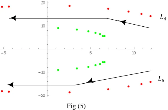
when 𝑦 ≠ 0 and the solutions of these two equations are given in figure (5) for different value of µ and mass reduction factor 𝛾. This figure (5) shows that there exist two non-collinear equilibrium points 𝐿4 and 𝐿5.We have observed that the mass reduction factor has a significant effect on the position of the non-collinear equilibrium points.
L1, .60 L1, .45 L1, .045
L1, .0045
L2, .60 L2, .45 L2, .045
L2, .0045
1.1 1.0 0.9 0.8 0.7 0.6 L1 0.1 0.2 0.3 0.4 0.5
0.7 0.6 0.5 0.4
L2 0.1 0.2 0.3 0.4 0.5
L3, .60 L3, .45 L3, .045
1.8 2.0 2.2 2.4 2.6 2.8 3.0
L3
0.1 0.2 0.3 0.4 0.5
1 1 2 3 Li
0.1 0.2 0.3 0.4 0.5 𝐿1 𝐿2
Fig (5)
In this fig (5) the green dot denotes the location of the ncep when 𝛾 = .6 and for various values of µ and red dot denotes the location of the ncep when 𝛾 = .45 and for various values of µ.
We have found that these points move from the right to left as µ increases and these points also moves away from the primaries as 𝛾 decreases.
4. Conclusion
In this paper, we have studied the magnetic binary problem when the infinitesimal body is of variable
mass. We have obtained the desired equations of motion and have also found the location of the collinear and
non-collinear equilibrium points. We have observed that there exist three collinear and two non-collinear
equilibrium points. We have found that that the points 𝐿1 and 𝐿2 move towards the origin whereas the point 𝐿3 go away from the origin as µ increases. We have also observed that the these points have the different positions for different values of mass reduction factor 𝛾 and small values of µ and for 𝐿1 and 𝐿2 this variation tends to zero as µ increases and 𝛾 decreases but for 𝐿3 this variation increases as µ increases and 𝛾 decreases. We have also observed
that the mass reduction factor has a significant effect on the position of the non-collinear
equilibrium points.
Conflict of Interests
The authors declare that there is no conflict of interests.
5 5 10
20 10 10 20
𝐿4
REFERENCES
[1] Mohd. Arif. Motion of a charged particle when the primaries are oblate spheroids, Int. J. Applied Math. Mech. 6(4) (2010), 94-106.
[2] K. Deimling, Zeros of accretive operators, Manuscripta Math. 13 (4) (1974), 365-374.
[3] Mohd. Arif. Motion around the equilibrium points in the planar magnetic binaries, Int. J. Applied Math. Mech. 9(20) (2013), 98-107.
[4] Mohd. Arif.A Study of the Equilibrium Points in the Photogravitational Magnetic Binaries Problem. Int. J. Modern Sci. Eng. Tech., 2 (11) (2015), 65-70.
[5] M.R. Hassan, Sweta,kumara, Md Aminul, Hassan. Existence of Equilibrium Points in the R3BP with Variable Mass When the Smaller Primary is an Oblate Spheroid. Int. J. Astron. Astroph. 7 (2017), 45-61.
[6] Jagadish Singh. Photogravitational restricted three body problem with variable mass, Indian. J. Pure. Appl. Math. 34 (2) (2003), 335-341.
[7] Jagadish Singh. Nonlinear stability of equilibrium points in the restricted three-body problem with variable mass, Astroph. Space Sci. 314 (4) (2008), 281-289.
[8] J.H. Astronomy and Cosmogony. Cambridge University Press, Cam-bridge (1928).
[9] Lukyanov, L.G.The Stability of the Libration Points in the Restricted Three-Body Problem with Variable Mass. Astron. J. 67(1990), 167-172.
[10] Mavraganis A. Motion of a charged particle in the region of a magnetic-binary system. Astroph. and Space Sci. 54(1978), 305-313.
[11] Mavraganis A. The areas of the motion in the planar magnetic-binary problem. Astroph. Space Sci. 57 (1978), 3-7.
[12] Mavraganis A. Stationary solutions and their stability in the magnetic -binary problem when the primaries are oblate spheroids. Astron. Astrophys. 80(1979), 130-133.
[13] Mavraganis. A. and Pangalos. C. AParametric variations of the magnetic -binary problem, Indian J. Pure Appl. Math. 14(3) (1983), 297- 306.
Astronomy, 8 (1963), 127.
[15] Shrivastava, A.K. and Ishwar, B. Equations of Motion of the Restricted Problem of Thre Bodies with Variable Mass. Celestial Mech. Dyn. Astron. (1983), 30, 323-328.