Simulation of Combustion and Thermal Flow inside an Industrial Boiler

University of New Orleans Theses and

Dissertations Dissertations and Theses

5-8-2004

Simulation of Combustion and Thermal Flow inside an Industrial

Simulation of Combustion and Thermal Flow inside an Industrial

Boiler

Boiler

University of New Orleans

Follow this and additional works at: https://scholarworks.uno.edu/td

Recommended Citation Recommended Citation

Saripalli, Raja, "Simulation of Combustion and Thermal Flow inside an Industrial Boiler" (2004). University of New Orleans Theses and Dissertations. 169.

https://scholarworks.uno.edu/td/169

This Thesis is protected by copyright and/or related rights. It has been brought to you by ScholarWorks@UNO with permission from the rights-holder(s). You are free to use this Thesis in any way that is permitted by the copyright and related rights legislation that applies to your use. For other uses you need to obtain permission from the rights-holder(s) directly, unless additional rights are indicated by a Creative Commons license in the record and/or on the work itself.

A Thesis

Submitted to the Graduate Faculty of the University of New Orleans in partial fulfillment of the requirements for the degree of

Master of Science in

The Department of Mechanical Engineering

by

Raja Saripalli

B.Tech, J.N.T.U, India, 2001

ii

iii

coordination, valuable suggestions, instructions via classes and productive discussions with

Dr.Wang has helped me and inspired me towards the successful completion of this task.

I would also like to take this opportunity to thank Dr.Carsie A Hall and Dr.Kazim M

Akyuzlu for serving on my defense committee.

I extend my special thanks to my family members, ECCC staff, and friends for their

iv

TABLE OF CONTENTS

List of Figures ... vi

List of Tables ... viii

Nomenclature ... ix

Abstract ... xi

1. Introduction...1

1.1 Background ...1

1.2 Objectives ...3

2. Literature Survey ...4

2.1 Boiler ...4

2.2 Combustion ...8

2.3 Pollutants ...9

2.4 NOx ...10

3. Problem Setup and Modeling...24

3.1 Governing Equations ...29

3.2 Computational Domain ...31

3.3 Turbulence Model ...35

3.4 Radiation Model ...42

3.5 Combustion Model ...43

3.6 Modeling and Calculation of NOx Emissions...45

4. Computational Method ...52

4.1 Fluent Background ...52

4.2 Solution Methodology ...53

4.3 Computational Grid ...55

4.4 Combustion Model ...55

4.5 Numerical Procedures ...57

4.6 Grid Independence Study ...62

5. Results...66

v

vi

LIST OF FIGURES

Figure 2.1 Fire tube and water tube boiler...7

Figure 2.2 Fuel NOx mechanism ...14

Figure 2.3 NO production associated with Fenimore prompt mechanism ...16

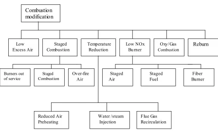
Figure 2.4 Combustion modification technologies for NOx control ...19

Figure 2.5 Low NOx burner employing air and fuel staging...22

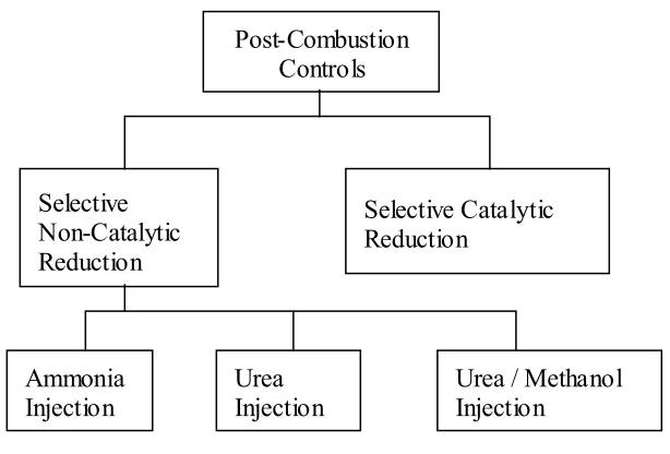
Figure 2.6 Post-combustion control technologies for NOx reduction ...23

Figure 3.1 3-D view of the studied boiler ...25

Figure 3.2 (a) Top view of the horizontal mid plane of the boiler...26

Figure 3.2 (b) Side view of the boiler ...27

Figure 3.2 (c) Compressed end view looking towards the burner ...27

Figure 3.3 Schematic and simulated burner geometry...28

Figure 3.4 Computational model of the 3-D view of burner exit ...29

Figure 3.5 Computational domain and boundary conditions for stage 1 ...32

Figure 3.6 (a) Computational domain for combustion chamber with boundary conditions for stage-2 study ...33

Figure 3.6 (b) Computational sub-domain with boundary conditions for the saturating and superheating regions ...33

Figure 3.7 A representative computational sub-domain with boundary conditions for the saturating and superheating regions in stage-2 simulation...34

Figure 3.8 Computational domain with boundary conditions for the chimney section in stage-3 simulation...35

Figure 4.1 Organizational program structure of FLUENT ...53

Figure 4.2 Computational model of the studied boiler showing different sections with meshes...56

Figure 4.3 Flow chart showing the segregated solution method ...59

Figure 4.4 Plot showing iterations of converged residuals ...61

Figure 4.5 Contours of temperature on horizontal plane y=0 for different meshing...63

Figure 4.6 Concentrations of CH4 and CO2 at different axial planes for different grids ...64

Figure 4.7 Profiles of velocity and temperature at different axial planes for different grids ...65

Figure 5.1 Velocity vectors for the three inlets in the burner ...67

Figure 5.2 Contours of static temperature on the vertical plane at x=0...70

Figure 5.3 Contours of static temperature on the horizontal plane at y=0...70

Figure 5.4 Contour temperature profile distribution on different horizontal y-planes ...71

vii

Figure 5.10 Contours of mass fraction of CH4, H2O, O2, CO2, and N2 on plane y=0 ...75

Figure 5.11 (a) Profiles of CH4 and O2 concentrations along selected axial distances...76

Figure 5.11 (b) Profiles of CO2 and H2O concentrations along selected axial distances...77

Figure 5.12 Contour temperature profile on the vertical center plane x=0 in the second stage simulation...79

Figure 5.13 Contour temperature profile on the horizontal center plane y=0 in the second stage simulation...79

Figure 5.14 Contour temperature plot at outlet of first section of the second stage ...80

Figure 5.15 Temperature contour plots on different y planes...81

Figure 5.16 Velocity vectors inside the first sub-section of the superheater section...82

Figure 5.17 (a) Temperature contour plot of the superheater tubes section including all the 31 sub-sections on the horizontal plane at y=0.3...84

Figure 5.17 (b) Profiles of mass-weighted average total pressure and temperature of all the 31 sub-sections on the horizontal plane at y=0.3...85

Figure 5.18 Contour plot of static pressure on different x-planes ...87

Figure 5.19 Contour plot of static pressure on different y-planes ...88

Figure 5.20 Contour plots of static pressure and velocity at the outlet of the boiler chimney ...88

Figure 5.21 Contour plots of static temperature at the outlet of the boiler chimney (a) simulated boiler chimney outlet, temperature is in (K) ...89

(b) Infrared thermography inspection of the boiler, temperature unit is in (F) ...89

Figure 5.22 Path lines colored by velocity magnitude on z-plane ...90

Figure 5.23 Vector plot colored by temperature on different y-planes...91

Figure 5.24 Vector plot colored by temperature on z-plane ...92

Figure 5.25 Contours of NO-ppm and NO mass fraction at vertical planes y = 0...94

Figure 5.26 Contours of NO-ppm and NO mass fraction on horizontal plane x = 0...95

viii

LIST OF TABLES

Table 4.1 Variables for three grids ...63

Table 5.1 Average velocities at the burner inlets...67 Table 5.2 Mass weighted pressure, temperature and velocity compositions at

inlets and outlets for all the 31 sub-sections in the saturator/superheater

ix

NOMENCLATURE

a Local speed of sound (m/s, ft/s)

c Concentration (mass/volume, moles/volume)

cp, cv Specific heat at constant pressure, volume (J/kg-K, Btu/lbm-°F) d Diameter (m, ft)

DH Hydraulic diameter (m, ft)

Dij Mass diffusion coefficient (m2 /s, ft2 /s)

E Total energy, activation energy (J, kJ, cal, Btu) f Mixture fraction (dimensionless)

g Gravitational acceleration (m/s2 , ft/s2 )

Gr Grashof number =

2 3 L ) T s T ( g ν ∞ − β (dimensionless)

H Total enthalpy (energy/mass, energy/mole) h Heat transfer coefficient (W/m2 -K, Btu/ft2 -h-°F) h Species enthalpy

h0 Standard state enthalpy of formation (energy/mass, energy/mole)

I Radiation intensity (energy per area of emitting surface per unit solid angle) J Mass flux; diffusion flux (kg/m2-s, lbm/ft2 -s)

K Equilibrium constant = forward rate constant/backward rate constant (units vary) k Kinetic energy per unit mass (J/kg, Btu/lbm)

k Reaction rate constant, e.g., k1, k-1,kf;r , kb;r (units vary) k Thermal conductivity (W/m-K, Btu/ft-h-°F)

kB Boltzmann constant (1.38 x10- 23 J/mole-K) k,kc Mass transfer coefficient (units vary) l, L Length scale (m, cm, ft, in)

m Mass (g, kg, lbm) •

m Mass flow rate (kg/s, lbm/s) Mw Molecular weight (kg/kgmol)

M Mach number = ratio of fluid velocity magnitude to local speed of sound Nu Nusselt number ≡

k hL

(dimensionless) p Pressure (Pa, atm, mm Hg, lbf /ft2) Pr Prandtl number =

α ν

(dimensionless) Q Flow rate of enthalpy (W, Btu/h) q Heat flux (W/m2 , Btu/ft2-h)

x r Radius (m, ft)

R Reaction rate (units vary) Re Reynolds number ≡

ν

VL

(dimensionless)

S Total entropy (J/K, J/kgmol-K, Btu/lbmol-°F) s Species entropy

s0 standard state entropy (J/kgmol-K, Btu/lbmol-°F)

Sc Schmidt number = D

ν _{(dimensionless)}

Sij Mean rate-of-strain tensor (s-1) T Temperature (K, °C, °R, °F) t Time (s)

U Free-stream velocity (m/s, ft/s)

u; v; w Velocity magnitude (m/s, ft/s); also written with directional sub-scripts (e.g., vx, vy, vz, vr)

V Volume ( m3, ft3)

vr Overall velocity vector (m/s, ft/s) X Mole fraction (dimensionless) Y Mass fraction (dimensionless)

α Permeability, or flux per unit pressure difference (L/m2-h-atm, ft3/ft2-h-(lbf/ft2)) α Thermal diffusivity (m2/s, ft2/s)

α Volume fraction (dimensionless) β Coefficient of thermal expansion (K- 1 ) γ Porosity (dimensionless)

γ Specific heat ratio, cp/cv (dimensionless)

∆ Change in variable, final - initial (e.g., ∆p, ∆t, ∆H, ∆S, ∆T) δ Delta function (units vary)

ε Emissivity (dimensionless)

ε Turbulent dissipation rate (m2/s3, ft2/s3)

η′′

η′ Rate exponents for reactants, products (dimensionless)

r

θ Radiation temperature (K)

ν Dynamic viscosity (cP, Pa-s, lbm/ft-s)

µ Kinematic viscosity (m2/s, ft2 /s)

ν ′′

ν′, Stoichiometric coefficients for reactants, products (dimensionless)

ρ Density (kg/m3, lbm/ft3)

σ Stefan-Boltzmann constant (5.67 x10 -8 W/m2-K4) s

σ Scattering coefficient (m-1) ≈

τ Stress tensor (Pa, lbf /ft2)

τ Shear stress (Pa, lbf /ft2)

τ Time scale, e.g., τc,τp,τc (s)

xi

operation of the superheater for producing high-pressure, high-temperature steam may result in

problems frequently caused by ruptured superheater tubes. To make the boiler more efficient,

less emission and less prone to tube rupture problems, it is important to understand the

combustion and thermal flow behaviors inside the boiler. This study performs a detailed

simulation of combustion and thermal flow behaviors inside an industrial boiler.

The simulations are conducted using the commercial CFD package FLUENT. The 3-D

Navier-Stokes equations and five species transport equations are solved with the eddy-breakup

combustion model. Calculation of NOx is performed after obtaining a converged flow, thermal

and combustion solution. The results provide insight into the detailed thermal-flow and

CHAPTER ONE

INTRODUCTION

1.1 Background

During the past three decades, due to economic and environmental demands, engineers

had to focus on improving the efficiency of energy producing power generation systems and in

the meantime reduce their pollution emissions. Computer simulation is one of the best tools that

can be applied in search for optimal solutions.

Boilers are commonly used in industries to burn fuel to generate process steam and

electric power. A situation may arise in which a considerable amount of unburned fuel is being

picked up by the gas and carried out of the boiler; this is known in the industry as carryover. As a

result, unburned fuel may be blown out of the boiler, causing efficiency and emissions problems.

Poor emissions could be caused by unburned hydrocarbon (UHC) and non-uniform heating

induced by cold and hot spots, which produce CO and NOx respectively. Also a situation may

arise where the superheater tubes break due to excessive heating, which may lead to boiler

shutdown and thus increase the expenses incurred.

Steam that has been heated above the temperature corresponding to its pressure is said to

be “superheated”. This steam contains more energy than does saturated steam at the same

pressure and the heat added provides more energy for the turbine for conversion to electric

problems frequently caused by ruptured superheater tubes. The damage or rupture of the

superheater tubes may be caused by many possible reasons including, galvanic corrosion,

thermal contraction and expansion, composition of the combustion gases, accumulations of soot

outside the pipes, accumulation of slag inside the pipe or high temperature distribution above

material yield temperature and high thermal stress. The damage caused by high temperature can

be minimized by providing uniform combustion and temperature distribution and keep fouling

resistance low, Installation of soot-blowers to remove accumulated soot and other particulates,

and optimizing the combustion conditions.

To help industry improve boiler’s efficiency, reduce emissions, avoid rupture of

superheater tubes, and understand the thermal flow transport in the boiler, this study employs the

Computational Fluid Dynamics (CFD) scheme. CFD simulations could provide a clear picture of

what is happening at any point within the boiler, making it easy in most cases to identify the

problem and develop a solution. A CFD analysis provides fluid velocity, pressure, and

temperature values throughout the solution domain for problems with complex geometries and

boundary conditions. During the analysis, the geometry of the system or boundary conditions

such as inlet velocity and flow rate can be easily changed to view their effects on thermal-flow

patterns or species concentration distributions. CFD can also provide detailed parametric studies

that can significantly reduce the amount of experimentation necessary to identify problems and

1.2 Objectives

The objective of the study is to model and simulate the thermal flow behavior of an

industrial natural gas fired boiler. The boiler information is provided by Dynegy Gas Plant at

Venice, Louisiana. The gas flow and temperature distribution is simulated with the commercial

CFD package FLUENT (6.1.22). FLUENT is a finite volume CFD code for solving transport

equations of mass, momentum and energy conservation. The specific goals are

1. To develop an appropriate numerical model to simulate the combustion features in the

boiler.

2. To investigate the flow pattern and temperature distribution inside the boiler.

3. To study the flow behavior and heat transfer near the superheater tubes.

4. To study the flow and aerodynamic behavior through the chimney.

5. To calculate emissions NOx.

6. To identify means that can help improve boiler efficiency, reduce emissions and avoid

CHAPTER TWO

LITERATURE SEARCH

The literature search focuses on introducing fundamental functions, requirements and

classification of the boilers, combustion, and NOx formation mechanisms and reduction

technologies.

2.1 Boiler

A boiler is a closed vessel in which water, under pressure, is transformed into steam by

the application of heat. In the furnace, the chemical energy in the fuel is converted into heat and

this heat is transferred to water to convert to steam.

2.1.1 Requirements of an efficient boiler

The ideal, reliable, economic and efficient boilers will embodies the following features:

! Simplicity in construction, excellent workmanship, and materials conducive to low

maintenance cost.

! Design and construction to accommodate expansion and contraction properties of

materials.

! Adequate steam and water space, delivery of clean steam, and good water circulation.

! A furnace setting conducive to efficient combustion and maximum rate of heat transfer.

! Should have low initial cost, installation cost and maintenance cost.

! Should be compact.

! Easy accessibility for cleaning and repair.

A boiler is designed to absorb the maximum amount of heat released in the process of

combustion. The heat is transmitted to the boiler by radiation, conduction and convection, the

percentage of each depending upon the boiler design.

2.1.2 Steam Utilization

Steam is generated for the following plant uses:

1. Driving turbine for electric generating equipment, blowers and pumps.

2. Process for direct contact with products, direct contact sterilization and non-contact for

processing temperatures for drying and sterilization.

3. Heating and air conditioning via absorption chillers for comfort and equipment.

4. Providing processing steam for water-shift reaction and other chemical process.

The efficiency achievable with steam generation relies heavily on the system's ability to

return condensed steam to the operating cycle. Many of the systems described above return a

significant portion of the condensed steam to the generation cycle.

2.1.3 Classification of boilers

Boilers are manufactured in many different sizes and configurations depending on the

a) Method of transporting hot gases:

On this basis, boilers can be classified as: Fire tube boiler and water tube boiler.

Fire tube boiler

In a fire tube boiler, hot gases pass through the tubes and water surrounds them. Heat

from the gases (produced by combustion) is transferred to water, which is then converted to

steam. Examples: Cochran, Lancashire, Cornish, Locomotiveboilers

Water tube boilers

In water tube boiler, water flows inside the tubes and the hot gases flow outside the tubes.

Examples: Babcock and Wilcox boiler(which has straight but inclined water tubes); Stirling

boiler(which has bent water tube).

Fire tube boilers need stronger outer shell to contain steam pressure, water tube boilers

does not need that.

b) Method of firing:

Internally fired: Furnace region is provided inside the boiler shell and is completely surrounded

by water-cooled surfaces. e.g., Lancashire, Locomotive boilers.

Figure 2.1 a) Fire tube boiler (above) b) Water tube boiler (below)

c) Pressure of steam:

Low pressure boiler: Steam pressure below 80 bars.

Examples: Cochran, Cornish, Lancashire, locomotive boilers

High pressure boiler: Pressure above 80 bars.

Examples: Lancashire, Locomotive, and Babcock & Wilcox boilers.

Forced circulation: Circulation of water takes by forced convection.

2.2 Combustion

Combustion occurs in boilers, refineries, drying kilns, incinerators, industrial ovens and

is also used to generate energy from biomass (e.g. from wood, straw, organic waste).

Combustion is the process whereby oxygen reacts with fuel, resulting in the release of heat and

light. The effectiveness of combustion can be measured by analyzing the flue gas and the amount

of soot. Perfect combustion is obtained when the flue gas analysis shows no carbon monoxide,

hydrogen or oxygen and when the percentage of carbon dioxide is at a maximum.

There are several factors or parameters that will affect combustion of heavy fuels in a

boiler:

1. Design of the combustion chamber

2. Design of the burner(s)

3. Condition of the burner(s)

4. Air and fuel ratio. Excess air of a few percent is normal

5. How well the air and fuel are mixed

6. Temperature and air speed in the combustion chamber

7. Air and fuel preheating

9. Chemical properties of the oil (asphaltenes, waxes, metal content)

10. Fuel droplet size if liquid fuels are used.

The combustion process provides tremendous amount of energy from a fuel and this

energy is converted or transformed to heat for cooking, making hot water, generating steam for

manufacturing or turning a turbine to produce shaft power and electricity, producing mechanical

motion as in an auto engine, or thrust as in an aero-engine.

The combustion of fuels requires the consumption of a large quantity of air. For example,

150 Lbs of a fuel (oil) requires about 2000 Lbs of air and resulting to 250 Lbs of CO2. Small

quantities of pollutants such as NO, CO and hydrocarbons are also formed, these quantities being

negligible from engineering calculations standpoint but very significant from the environmental

standpoint.

The combustion process involves some 1000 reactions to complete the oxidation process

forming CO2 and H2O, the ultimate products of combustion. However, pollutants such as CO,

unburned hydrocarbons (UHC), soot, NOx, SO2 are also formed during the combustion process

as a result of the various reactions.

2.3 Pollutants

Control of pollutant emissions is a major factor in the design of modern combustion

system. Pollutants of concern include (i) particulate matter such as soot, fly ash, metal fumes,

various aerosols etc, (ii) the sulfur oxides SO2 and SO3, (iii) unburned and partially burned

hydrocarbons such as aldehydes, and (iv) oxides of Nitrogen, NOx which consists of NO and

are those formed via reactions involving primary pollutants in the atmosphere.

Four major negative effects of pollutants are

1. Altered properties of the atmosphere and precipitants

2. Harm to vegetation

3. Foiling and deterioration of materials

4. Potential increase of morbidity and mortality in humans

5. Depleting ozone layer

6. Affecting Global warming

7. Producing Acid rains

2.4 NOx

NOx emission consists of mostly nitric oxide (NO). It also contains nitrogen oxide (NO2)

and nitrous oxide (N2O). NOx is a precursor for photochemical energy and contributes to acid

rain and causes ozone depletion. The quantity of NOx formed depends on three T’s :

Temperature, Time, and Turbulence.

Oxides of Nitrogen Formation:

In every circumstance where combustion occurs, the formations of nitrogen oxides (NOx)

are inevitable. From a home open fire to a coal fired power plant, NOx is formed as an undesired

NOx is used to refer to NO and NO2. NO is the primary form in combustion products

(typically 95 percent of total NOx). NO is subsequently oxidized to NO2 in the atmosphere.

Nitrogen Oxide Formation occurs through three reaction paths, each having unique

characteristics which is responsible for the formation of NOxduring combustion processes:

(1) Thermal NOx, which is formed by the combination of atmospheric nitrogen and

oxygen at high temperatures;

(2) Fuel NOx, which is formed from the oxidation of fuel-bound nitrogen; and

(3) Prompt NOx, which is formed by the reaction of fuel-derived hydrocarbon fragments with atmospheric nitrogen in an early phase of the flame front.

NOx emissions do not form in significant amounts until flame temperatures reach 2800 F.

Once that threshold is passed, any further rise in temperature causes a rapid increase in the rate

of NOx formation. Lower excess air levels (fuel rich) starve the reaction for oxygen, and higher

excess air levels (lean burn) drive down the flame temperature, slowing the rate of reaction.

In the combustion of fuels that contains no nitrogen, nitric oxide is formed by three

chemical mechanisms:

1. The Thermal or Zeldovich Mechanism

2. The Prompt or Fenimore Mechanism

NOx is produced during the combustion process when nitrogen and oxygen are present at

elevated temperatures. The two elements combine to form NO or NO2. NOx is generated by

many combustion processes. It combines with other pollutants in the atmosphere and creates O3,

a substance known as ground level ozone.

The formation of thermal mechanism dominates in high-temperature combustion over a

fairly wide range of equivalence ratios. Equivalence ratio is defined as the ratio of actual fuel/air

ratio over the theoretical fuel/air ratio. The formation of thermal NOx is determined by a set of

highly temperature-dependent chemical reactions known as the extended Zeldovich mechanism.

The principal reactions governing the formation of thermal NOx from molecular nitrogen are as

follows:

O + N2 ⇔ NO + N (2.4.1)

N + O2 ⇔ NO + O (2.4.2)

A third reaction, particularly at near-stoichiometric conditions and in fuel-rich

mixtures which contributes to the mechanism is

N + OH ⇔ NO + H (2.4.3)

The activation energy for first reaction (2.4.1) is relatively large, 319,050 kJ/kmol.

Therefore this reaction has very strong temperature dependence. The thermal mechanism is

processes, NO is formed rather slowly by thermal mechanism; thus, thermal NO is generally

considered to be formed in post flame gases.

2.4.2 Fuel NOx Formation

Fuel NOX formation is a more complex process involving local concentration of oxygen

and nitrogen and is reduced by minimizing the availability of oxygen during various stages of the

combustion process. Fuel-bound NOx is generated from nitrogen compounds present in the fuel

itself. Gaseous fuels, such as natural gas or propane, are free of nitrogen compounds. However,

fuel oils and coal can contain significant amounts of fuel-bound nitrogen. During combustion,

the conversion rate of fuel-bound nitrogen to NOx varies widely over a range of 20 to 70%.

During combustion process, nitrogen-containing organic compounds present in liquid or

solid fossil fuel contributes to the total NOx formed. The fuel nitrogen is a particularly important

source of nitrogen oxide emissions for residual duel oil, coke, and coal, which typically contain

0.3-2% nitrogen by weight. The fuel-bound NOx contribution depends on the amount of nitrogen

that is chemically bound in the fuel. The fuel NOx formation is generally important in

non-premixed combustion. The fuel NOx formation is not important in non-premixed combustion

applications since most fuels used in premixed combustion contain little or no bound nitrogen.

Under the reducing conditions surrounding the burning droplets or particles, the

fuel-bound nitrogen is converted to fixed nitrogen species such as HCN and NH3. These, in turn, are

readily oxidized to form NO if they reach the lean zone of the flame. Between 20 and 80 percent

Fuel Nitrogen

NH3

HCN

NO

N2

NO

NO O2

O2

Figure 2.2 Fuel NOx mechanism

2.4.3 PROMPT NOx Formation

Prompt NOx is the third and least significant NOx formation mechanism. In this

mechanism, nitrogen from combustion air reacts with hydrocarbon radicals from the fuel to form

a hydrogen cyanide intermediate. The hydrogen cyanide then reacts with oxygen and nitrogen in

combustion air to form nitrogen oxide.

Hydrocarbon fragments (such as C, CH, CH2) may react with atmospheric nitrogen under

fuel-rich conditions to yield fixed nitrogen species such as NH, HCN, H2CN, and CN. These, in

nitrogen-containing fuels, the prompt mechanism is responsible for only a small fraction of the

total NOx. Its control is important only when attempting to reach the lowest possible emissions.

The formation of prompt NOx is governed by a set of equations known as Fenimore

mechanism. The scheme of Fenimore mechanism is that hydrocarbon radicals react with

molecular nitrogen to form amines or cyano compounds. The amines and cyano compounds are

then converted to inverted compounds that ultimately form NO. The Fenimore mechanism is

given as:

CH + N2 ⇔ HCN + N (2.4.4)

C + N2⇔ CN + N (2.4.5)

N + O2⇔ NO + O (2.4.6)

HCN + OH ⇔ CN + H2O (2.4.7)

N + OH ⇔ NO + H (2.4.8)

In the atmosphere, nitric oxide ultimately oxidizes to form nitrogen oxide, which

contribute to production of acid rain and photochemical smog. Production of NO associated with

F

igure 2.3 NO production associated with Fenimore prompt mechanism

Prompt NOx formation is proportional to the number of carbon atoms present per unit

volume and is independent of the parent hydrocarbon identity. The quantity of HCN formed

increases with the concentration of hydrocarbon radicals, which in turn increases with

equivalence ratio. As the equivalence ratio increases, prompt NOx production increases, then

passes a peak, and finally decreases due to deficiency in oxygen.

2.4.4 NOx Formation From Reburning

In Reburning NO mechanism, NO reacts with hydrocarbons and is subsequently reduced.

In general the mechanism is given as

CHi + NO –→HCN + products (2.4.9)

NCO NH

HCN

Fuel-N HNCO

NO N2

N2

O

OH H

H O2

NH2

H2O

H2

O

OH OH

OH

OH H

Three reburn reactions for temperature range 1600 ≤ T≤ 2100 are

CH + NO –K1→ HCN + O (2.4.10)

CH2 + NO –K2→ HCN + OH (2.4.11)

CH3 + NO –K3→ HCN + H2O (2.4.12)

Where K1, K2 and K3 are rate constants for the above reactions

K1 = 1 * 108 [m3 / gmol-s]

K2 = 1.4 * 106 * e-550/T [m3 / gmol-s]

K3 = 2 * 105 [m3 / gmol-s]

2.4.5 NOx Control

NOx control technologies currently used within the industry can be grouped into two

categories i.e combustion modifications and post-combustion NOx control technologies. The

first addresses reducing the production of NOx by making changes in the combustion process or

the fuel stream. The second involves mitigating the NOx that has been produced by the

application of post-combustion technology through the use of chemical reagents. For coal-fired

applications, combustion system modifications are generally less costly and may independently

result in emissions levels that satisfy regulatory requirements. Several methods are available to

effectively limit NOx formation during combustion. The optimum combustion system redesign

may blend several of these, selected on the basis of unit capacity and fuels to be fired and of

applicable NOx reduction requirements.

For processes dominated by thermal NOx formation, time, temperature, and oxygen

recirculated flue gas to the combustion air to depress flame temperature.

Fuel NOx formation can be reduced by switching to, or co-firing with, fuel with lower

nitrogen content and/or by limiting oxygen availability during the early stages of combustion.

Oxygen reduction mechanisms include reducing excess air, reducing burner stoichiometry by

removing a portion of the combustion air from the burner zone and introducing this air later

through NOx or overfire air (OFA) ports (air staging), and limiting the rate that air is introduced

to the fuel during the early stages of combustion with specially designed burners.

Combustion Modifications for NOx control

Low Excess Air ---- Reducing the air supplied in the furnace lowers NOx production. Thermal

NOx emissions peak at leaner than stoichiometric equivalence ratios. The NOx creation rate

typically peaks at excess oxygen levels of 5-7% where the combination of high combustion

temperatures and the higher oxygen concentration act together. At both lower and higher air/fuel

ratios, NOx production falls off due to lower flame temperature at high excess air levels and

lower oxygen at low air levels. Low air is achieved by changes in operating procedures, system

controls or both. The NOx reduction technique involves reducing the air supplied. Only limited

NOx reductions are possible when low air level is supplied because excessive reduction in air

Combustion modification Low Excess Air Staged Combustion Temperature Reduction Low NOx Bu rner Oxy/Gas

Combustion Reburn

Burners out of service Staged Combustion Over-fire Air Staged Air Staged Fuel Fiber Burner Reduced Air Preheating Water /steam Injection Flue Gas Recirculat ion

Figure 2.4 Combustion modification technologies for NOx control

Staged Combustion — Staged combustion processes significantly reduce NOx emissions. In the

initial stage of combustion, the air supplied to the burners is less than the amount required to

completely burn the fuel. During this stage, fuel-bound nitrogen is released but cannot be

oxidized, so it forms stable molecules of harmless molecular nitrogen (N2). Other components of

the fuel are also released without being fully oxidized. These include carbon particles and carbon

monoxide. By adding a second stage, in the air-fuel mixture, the carbon and carbon monoxide

can be burned, converting them to carbon dioxide.

Over-fire Air — Over-fire air is the air that is injected into the furnace above the normal

combustion zone. Generally when Over-fire air is employed, the burners are operated at a lower

Flue Gas Recirculation — Flue Gas Recirculation, in which part of the flue gas is recirculated

to the furnace, can be used to modify conditions in the combustion zone (lowering the

temperature and reducing the oxygen concentration) to reduce NOx formation. Flue Gas

Recirculation is also used as a carrier to inject fuel into a reburn zone to increase penetration and

mixing.

Operational Modifications — Changing certain boiler operational parameters can create

conditions in the furnace that will lower NOx production. Examples include

burners-out-of-service (BOOS), low excess air (LEA), and biased firing (BF). In BOOS, selected burners are

removed from service by stopping fuel flow, but airflow is maintained to create staged

combustion in the furnace. LEA involves operating at the lowest possible excess air level

without interfering with good combustion, and BF involves injecting more fuel to some burners

(typically the lower burners) while reducing fuel to other burners (typically the upper burners) to

create staged combustion conditions in the furnace.

Low NOx Burners (LNB) — Low NOx Burners are designed burners to control the mixing of

fuel and air to achieve what amounts to staged combustion. This staged combustion reduces both

flame temperature and oxygen concentration during some phases of combustion, in turn, reduces

both thermal NOx and fuel NOx production. The most common LNB types achieve lower NOx

emissions by "staging" the injection of either air or fuel in the burner region. Low NOx burners

are classified as either a staged air or a staged fuel burner. Air staging is more common. As the

regions along the flame front. These regions are typically referred to as the primary, secondary

and tertiary (staged) air zones. The division of combustion air reduces the oxygen concentration

in the primary burner combustion zone, lowering the amount of NO formed there and increasing

the amount of NO-reducing agents formed in an oxygen deficient combustion zone. Secondary

and tertiary air injections complete the combustion downstream of the primary zone, lowering

the peak temperature and reducing thermal NOx formation. Aside from the basic staged air

burner, there are other variations of staged air burners that incorporate internal recirculation of

combustion products to aid in NOx reduction. Low NOx Burners are often coupled with over fire

(secondary) air (OFA) injection to assure complete combustion. Low NOx burner employing air

staging and fuel staging is shown in Figure 2.5.

Reburning — In the Reburning process, part of the boiler fuel input (typically 10-25%) is added

in a separate reburn zone. The fuel-rich reducing conditions in this zone lead to the reduction of

NOx formed in the normal combustion zone. OFA is injected above the reburn zone to complete

combustion. Thus, with reburn there are three zones in the furnace: (1) a combustion zone with

an approximately normal air-to-fuel ratio; (2) a reburn zone, where added fuel results in a

fuel-rich condition; and (3) a burnout zone, where OFA completes the combustion. Coal, oil, or gas

Figure 2.5 (a) Low NOx burner employing air staging (above)

Post-Combustion controls for NOx reduction

The post-combustion controls can be achieved by using selective non-catalytic reduction

(SNCR) and selective catalytic reduction (SCR) as shown in Figure 2.6.

Post-Combustion Controls

Selective Non-Catalytic Reduction

Selective Catalytic Reduction

Ammonia

Injection Urea Injection Urea / Methanol Injection

Figure 2.6 Post-combustion control technologies for NOx reduction

Selective Non-Catalytic Reduction (SNCR) — In this post control technique, a nitrogen

containing additive, ether ammonia, urea, or cyanuric acid is injected and mixed with flue gases

to affect chemical reduction of NO to N2 without the aid of catalyst. Temperature is a critical

variable, and operation within a relatively narrow range of temperatures is required to achieve

large NOx reductions.

Selective Catalytic Reduction (SCR) — In this technique, a catalyst is used in conjunction with

ammonia injection to reduce NO to N2. Effective reduction depends on the temperature range

and is about 480 K to 780 K. Greater NOx reductions are possible but the costs of NOx removal

are generally the highest of all NOx control techniques because of both the initial cost and the

CHAPTER THREE

PROBLEM SETUP AND MODELING

The overall design of the studied boiler is shown in Figure 3.1. The model basically

consists of four sections, burner, combustion chamber, saturating/superheating, and chimney

(exhaust). The top view of the boiler is shown in Figure 3.2. The burner is provided with three

inlets, two for air inlet and one for fuel inlet. Primary and secondary air enters the burner as

shown in Figure 3.3 and Figure 3.4. The primary air enters with a swirl and is directed outward.

The air entering around the outside periphery of the swirl air is defined as the secondary air. It

contributes to a controlled expansion in the quarl section of the burner where it reacts with the

unburned fuel from the center reaction to complete the combustion process. The fuel used is

Methane, CH4, which is burned in the combustion chamber and the flue gasses pass through the

Exhaust

Chimney

Combustion

Chamber Walls

(shaded grey)

Burner

Inlet

Boiler Outer

Walls

Figure 3.1 A 3-D view of the studied boiler (steam tubes are not shown)

The problem is modeled with the following general assumptions:

1. The flow is steady and incompressible.

2. Variable fluid properties.

3. Turbulent Flow

4. Instantaneous combustion with the chemical reaction much faster than the turbulence

time scale.

5. The steam temperature is assumed as the tube wall temperature.

The full three-dimensional Navier-Stokes equations are employed with five species transport

Boiler outer wall made of saturator tubes

Boiler Outer Wall Boiler inner walls

Flame Flue Gases

Saturated water tubes

Burner

Gases to chimney

Gases to chimney

Superheater tubes 6x19 array x four passes Boiler wall made of alternating

superheater and saturator tubes (see details in Figure 3.)

4.125 ft

29.33 ft

11.8 ft 11.1 ft

22.9ft

Gasses to

atmosphere

Combustion

chamber

Burner

Drum

Prima ry A ir, enters with a sw irl Secondary Air

Fue l (metha ne)

Secondary Air

Primary Air with

swirl

Fuel Inlet

Secondary Air

Figure 3.4. Computational model of the 3-D view of the burner exit

3.1 Governing Equations

The conservation equations for mass, momentum and energy conservation in general form are

shown below.

0 ) v (

t + ∇ ⋅ ρ =

∂ρ ∂ (3.1) F g ) ( p ) v v ( ) v ( t r r r r

r _{+∇⋅ ρ =−∇ +∇⋅ τ +ρ +} ρ

∂

∂ _(3.2)

Sh ) v eff ( J j jh j T keff )) p E ( V ( ) E (

t +

       ⋅ τ + ∑ − ∇ ⋅ ∇ = + ρ ⋅ ∇ + ρ ∂

∂ r r r



 3

where I is the unit tensor.

In energy equation E is given as

2 v 2 p h

E +

ρ −

= (3.5)

“h” is sensible enthalpy and for incompressible flow it is given as

ρ + ∑

= _{h j} p

j Y j

h (3.6)

dT T

T ref c_p,j

h j= ∫ (3.7)

Tref is constant taken as 298.15 K

Sh in the energy equation (3.3) is the source term, which is provided by the net enthalpy

The boundary conditions are

Fuel inlet: Mass inlet condition , m. fuel =0.855 kg/s

Air inlet: m• primary air = 6.9 kg/s,

•

msecondary air = 13.08 kg/s

Outlet: Constant pressure outlet condition at P = 1 bar

Walls: Adiabatic or constant wall temperature

! Flow: No-slip condition at the walls; u = 0, v = 0, w = 0.

! Temperature: Walls at the surfaces inside the combustion chamber are covered by the saturating steam tubes at constant temperature at T = 526.68 K

! All the superheaters are set at the constant temperature at T = 672.03 K ! Saturator section: All walls set at T = 526.68 K

! Superheater section: Outer wall is at alternating saturator (T = 526.86 K) and superheater temperature (T = 672.03 K)

! Chimney walls: Adiabatic

3.2 Computational Domain

In view of the complex geometry of the boiler, the simulation is conducted in three

stages.

Stage 1: In this stage of study, the computational domain includes the entire boiler but excludes

water/steam tubes. The computational domain with all boundary conditions is shown in Figure

3.5.

Stage 2: In stage 2 of study, detailed simulation of the saturating and superheating regions is

performed. Due to the large numbers of saturator and superheater tubes, the simulation is broken

down into 33 sub-sections. Each sub-section includes 4x2x2 tubes. The geometry and boundary

condition for the saturating/superheating regions (Figure 3.7). A total of 32 sub-sections of

similar computational domain as shown in Figure 3.7 are simulated. Each uses the outlet profile

solution of the previous sub-section as the inlet profile boundary condition. In this approach the

inlet pressure information will be calculated and updated to satisfy overall mass and momentum

conservation.

Burner: Mass flow rates Fuel: 0.855 kg/s Primary air: 6.9 kg/s Secondary air: 13.08 kg/s

Outlet: Constant pressure P = 1 atm

Combustion chamber walls: Constant temperature T=526.68 K

Boiler outer walls: Constant temperature T = 526.68 K

Chimney: adiabatic

Burner

Combustion

chamber walls,

T=526.68 K

Alternating

saturator/superheator

tubes as the wall

Outlet,

pressure

condition

Saturator

wall,

T=526.68 K

Flow

Superheater tubes (marked red), T=672.03 K

Saturator tubes (marked white in between superheater tubes)

T=526.68 K

Pressure outlet, P=1 bar Outer drum wall, T=526.68 K Saturator wall,

T=526.68 K

Figure 3.6 (a) Computational domain for combustion chamber with boundary conditions for stage-2 study (b) Computational sub-domain with boundary conditions for the saturating and

Alternating saturator/superhea walls

Superheater tube T=672.03 K Saturator tubes,

T=526.68 K

Inner walls, T=526.68 K

Outer walls, T=526.68 K

Outlet, Pressure outlet, P= 1 bar

Flow

Figure 3.7 A representative computational sub-domain with boundary conditions for the saturating and superheating regions in stage-2 simulation

Stage 3: In this phase of study, the outlet results of stage 2 are used to calculate the flow in the

chimney section. For this stage the computational domain and boundary conditions are shown in

figure 3.8. The outlet profile (velocity, temperature and species concentration) solution of the last

Pressure outlet

condition

Velocity inlet

profile condition

Constant wall

temperature

condition

Adiabatic wall

condition

Figure 3.8 Computational domain with boundary conditions for the chimney section in stage-3 simulation

3.3 Turbulence Model

Turbulent flows are characterized by spectral broad-brand, randomly fluctuating velocity

fields. These fluctuations mix transported quantities such as momentum, energy, and species

concentration, and cause the transported quantities to fluctuate as well. Since these fluctuations

can be of small scale and high frequency, they are too computationally intensive to simulate

directly in practical engineering calculations. Instead, the instantaneous (exact) governing

equations can be time-averaged, ensemble-averaged, or otherwise manipulated to remove the

small scales, resulting in a modified set of equations that are computationally less expensive to

solve. However, the modified equations contain additional unknown variables, and turbulence

! κ-ε models

- Standard κ-ε model

- Renormalization-group (RNG) κ-ε model - Realizable κ-ε model

! κ-ω models

- Standard κ-ω model

- Shear-stress transport (SST) κ-ω model

! υ2-f model

! Reynolds stress model (RSM)

! Large eddy simulation (LES) model

In view of the complex flow field in the boiler, this study selects the standard κ-ε model

due to its suitability for a wide range of wall-bound and free-shear flows. The standard κ-ε model

is the simplest of turbulence two-equation model in which the solution of two separate transport

equations allows the turbulent velocity and length scales to be independently determined. The κ

-ε model is a semi-empirical model with several constants obtained from experiments.

All the three κ-ε models have similar forms, with major differences in the method of

calculating the turbulent viscosity, the turbulent Prandtl numbers, and the generation and

destruction terms in the k-ε equations.

The standard κ-ε model is a semi-empirical model based on model transport equations for

derived from the exact equation, while the model transport equation for ε is obtained using

physical reasoning and bears little resemblance to its mathematically exact counterpart.

The turbulence kinetic energy, κ, and its rate of dissipation, ε, are obtained from the

following transport equations:

k M b k j k t j i i S Y G G x x u x

t __+ + − − +

     ∂ ∂ + ∂ ∂ = ∂ ∂ + ∂ ∂ κ _ρε σ µ µ ρκ ρκ) ( ) ( )

( (3.8)

ε + κ ε ρ ε − ε + κ ε ε +         ∂ ε ∂ ε σ µ + µ ∂ ∂ = ρε ∂ ∂ + ρε ∂

∂ 2 _S

2 C ) b G 3 C k G ( 1 C j x ) t ( j x ) i u ( i x ) (

t (3.9)

In these equations, Gk represents the generation of turbulence kinetic energy due to the mean

velocity gradients and the Reynolds stress, calculated as

i j j i x u u u G ∂ ∂ − = −_ρ−−−'−'

κ (3.10)

b

G represents the generation of turbulence kinetic energy due to buoyancy, calculated as

i x T t Pr t i g b G ∂ ∂ µ β

= (3.11)

where Prt is the turbulent Prandtl number and gi is the component of the gravitational vector in

p T ∂ ρ

In equation (3.8), YM represents the contribution of the fluctuating dilatation in compressible

turbulence to the overall dissipation rate, and is given as

2 t M 2 M

Y = ρε (3.13)

where Mt is the turbulent Mach number, given as

2 a

k

Mt = (3.14)

where a = γRT is the speed of sound.

The turbulent (or eddy) viscosity, µt, is computed by combining κ and ε as

ε κ µ ρ =

µ_t C 2 (3.15)

C1ε, C2ε, Cµ, σκ, and σt are constants and have the following values

C1ε= 1.44, C2ε = 1.92, Cµ = 0.09, σκ = 1.0, σt= 1.3 (3.16)

These constant values have been determined from experiments with air and water for

grid turbulence. They have been found to work fairly well for a wide range of wall-bounded and

free-shear flows. The initial values for κ and ε at the inlets and outlet are set as 1 m2/s2 and 1

m2/s3 respectively.

In general, turbulent flows are significantly affected by the presence of walls. Very close

to the wall, viscous damping reduces the tangential velocity fluctuations, while kinematic

blocking reduces the normal fluctuations and away from the wall the turbulence is increased by

the production of turbulence kinetic energy. In the near-wall region the solution variables have

large gradients, and the momentum and other scalar transports occur strongly. Therefore,

accurate representation of the flow in the near-wall region is required for successful predictions

of wall-bounded turbulent flows.

The κ-ε turbulence model used in this study is primarily valid for turbulent core flows

(i.e., the flow in the regions somewhat far from walls). Wall functions are used to make this

turbulence model suitable for wall-bounded flows. Wall functions are a collection of

semi-empirical formulas and functions that link the solution variables at the near-wall cells and the

corresponding quantities on the wall. The wall functions consists of the following:

! Laws of the wall for mean velocity and temperature and other scalars

! Equations for near-wall turbulent quantities

The law-of –the-wall for mean velocity gives

) Ey ln( 1

U +

κ =

µ µ ρ ≡

+ C0.25k0P.5yP y

k = von Karman constant (=0.42)

E = empirical constant (=9.793)

UP = meanvelocity of the fluid at point P

kP = turbulence kinetic energy at point P

yP = distance from point P to the wall

µ = dynamic viscosity of the fluid

The logarithmic law for mean velocity is valid for y+ > about 30 to 60

The law-of-the-wall for temperature is given

) y y ( U ) Pr (Pr U {Pr q k C 5 . 0 ] P ) Ey ln( k 1 [ Pr ) y y ( U q k C Pr 5 . 0 y Pr q k C c ) T T ( T T 2 c t 2 P t 5 . 0 P 25 . 0 t T 2 P 5 . 0 P 25 . 0 5 . 0 P 25 . 0 p P w + + • µ + + + • µ + • µ + > − + ρ + + = < ρ + = ρ − ≡ (3.18)

where P is computed using the formula

        − +             −        

= 4 1 1 0.28e 0.007Pr/Prt 3 rt P r P 24 . 9

P (3.19)

kf = thermal conductivity of the fluid

ρ = density of fluid

•

q = wall heat flux

Tp = temperature at the cell adjacent to the wall

Tw = temperature at the wall

Pr = molecular Prandtl number (

f p c κ µ )

Prt = turbulent Prandtl number (=0.85 at the wall)

A = 26 (Van Driest constant)

κ = 0.4187 (von Karman constant)

E = 9.793 (wall function consatant)

Uc = mean velocity magnitude at y+ = yT+

For κ-ε turbulence model, wall adjacent cells are considered to solve the κ-equation. The

boundary condition for κ imposed at the wall is 0 n =

∂ κ ∂

, where “n” is the local coordinate normal

to the wall. The production of kinetic energy, Gk, and its dissipation rate, ε, at the wall-adjacent

cells, which are the source terms in κ equation, are computed on the basis of equilibrium

hypothesis with the assumption that the production of κ and its dissipation rate assumed to be

equal in the wall-adjacent control volume. The production of κ and ε is computed as

P y 5 . 0 P k 25 . 0 C w w y U w k G µ κρ τ τ = ∂ ∂ τ

≈ (3.20.a)

P y 5 . 1 p k 75 . 0 C

P = µ_κ

∫π Φ ⋅ Ω π σ + π σ = σ + + 4 0 ' d ) ' s s ( ) ' s , r ( I 4 s 4 T 2 an ) s , r ( I ) s a ( ds ) s , r (

dI r r _{r r r r r r}

(3.21.a)

where rr is position vector

s

r _{is direction vector}

'

s

r _{is scattering direction vector}

s is path length

a is absorption coefficient

n is refractive index

s

σ is scattering coefficient

I is radiation intensity, which depends on position rr and direction sr

T is local temperature

Φ is phase angle

'

Ω is solid angle

The Rosseland radiation model [7] is used in this study, which is valid for medium optical

thickness. The radiative heat flux in a gray medium is approximated by the following equation

G r

q =−Γ∇ (3.21.b)

where Γ is given as

) s C ) s a ( 3 ( 1 σ − σ + =

Γ (3.21.c)

4 T 4

In Rosseland model it is assumed that the intensity is the black-body intensity at the gas

temperature. Therefore substituting equation (3.21.d) into equation (3.21.b) gives

T 3 T 16 r

q =− σΓ ∇ (3.21.e)

3.5 Combustion Model

Modeling for combustion ranges from nonreacting to multiple reactions with multiple

species, and finite rate kinetics. In this study, combustion of methane is modeled by a single-step

reaction. The mixing and transport of chemical species is modeled by solving the conservation

equations describing convection, diffusion, and reaction sources for each component species.

The species transport equations are solved by predicting the local mass fraction of each species,

Yi, through the solution of a convection-diffusion equation for the i-th species. The species

transport equation in general form is given as:

( )

(

)

t +∇⋅ =−∇⋅ + +

∂

∂ _v r

ν ρ

ρ (3.22)

where Ri is the net rate of production of species i by chemical reaction. Si is the rate of creation

by addition from the dispersed phase plus any user-defined sources. Ji r

is the diffusion flux of

species i, which arises due to concentration gradients. Mass diffusion for laminar flows is given

as

i m i

i D Y

Jr =−ρ _, ∇ (3.23)

For turbulent flows, mass diffusion flux is given as

i t t m i i Y Sc D

J _∇

The reaction rate that appears as source term in equation (3.22) is given by the

turbulence-chemistry interaction model called the eddy-dissipation model. The overall rate of

reaction for most fast burning fuels is controlled by turbulent mixing. The net rate of production

of species i due to reaction r, Ri,r, is given by the smaller of the two given expressions below:

          ν κ ε ρ ν = R , w M r , R ' R Y R min A i , w M r ,i ' r ,i

R (3.25)

j , w M N

j " ,jr P PY AB i , w M r ,i ' r ,i R ∑ ν ∑ κ ε ρ ν

= (3.26)

where YP is the mass fraction of any product species, P

YR is the mass fraction of a particular reactant, R

A is an empirical constant equal to 4.0

B is an empirical constant equal to 0.5

r ,i '

ν is the stoichiometric coefficient for reactant “i” in reaction “r”.

r ,j "

In the above equations (3.25) and (3.26), the chemical reaction rate is governed by the

large-eddy mixing time scale,

ε

κ

, and an ignition source is not required. This is based on the

assumption that the chemical reaction is much faster than the turbulence mixing time scale, so

the actual chemical reaction is not important.

In this study, methane (CH4) is used as fuel. The complete stoichiometric combustion

equation is given below:

CH4 + 2(O2 + 3.76 N2)→ CO2 + 2H2O + 7.52 N2 (3.27)

3.6 Modeling and Calculation of NOx Emissions

NOx emission consists of mostly nitric oxide (NO). Less significant are nitrogen oxide,

NO2 and nitrous oxide (N2O). NOx is a precursor for photochemical smog, it contributes to acid

rain, and causes ozone depletion. Thus, NOx is a pollutant.

To predict NOx emission, transport equation for nitric oxide (NO) concentration are

solved. With fuel NOx sources, an additional transport equation for an intermediate species

(HCN or NH3) are solved. Since NOx concentrations generated in a combustion system are

generally low, NOx chemistry has negligible influence on the predicted flow fields, and species

concentrations. Therefore, the calculation of NOx concentrations can be post-processed after the

thermal flow and major species concentrations are computed.

The NOx transport equations are solved based on a given flow field and combustion

solution. NOx is post processed from a combustion simulation, thus an accurate combustion

development cost.

In laminar flames, and at the molecular level within turbulent flames, the formation of

NOx can be attributed to four distinct chemical kinetic processes: thermal NOx formation,

prompt NOx formation, fuel NOx formation, and reburning. Thermal NOx is formed by the

oxidation of atmospheric nitrogen present in the combustion air. Prompt NOx is produced by

high-speed reactions at the flame front, and fuel NOx is produced by oxidation of nitrogen

contained in the fuel. The reburning mechanism reduces the total NOx formation by accounting

for the reaction of NO with hydrocarbons.

The mass transport equation for the NO species is solved taking into account convection,

diffusion, production and consumption of NO and related species. The effect of residence time in

NOx mechanisms, a Lagrangian reference frame concept, is included through the convection

terms in the governing equations written in the Eulerian reference frame. For thermal and prompt

NOx mechanisms, only the NO species transport equation is needed which is given as

NO S ) NO Y D ( ) NO Y vˆ ( ) NO Y (

t ρ +∇⋅ ρ =∇⋅ ρ ∇ +

∂

∂ r

(3.28)

Thermal NOx

The formation of thermal mechanism dominates in high-temperature combustion over a

highly temperature-dependent chemical reactions known as the extended Zeldovich mechanism

described

O + N2 ⇔

f 1 k r 1 k

NO + N (3.29)

N + O2 _⇔

f 2 k r 2 k

NO + O (3.30)

N + OH k_⇔3f

r 3 k

NO + H (3.31)

The net rate of formation of NO via extended Zeldovich mechanism reactions described

above from equations (3.29) to (3.31) is given by

d[NO] / dt = K1f[O][N2] + K2f[N][O2] + K3f[N][OH] - K1r[NO][N] – K2r[NO][O]

- K3r[NO][H] (3.32)

Where all concentrations have units of gmol/m3. In order to calculate the formation rates

of NO and N, the concentrations of O, H, OH are required. The rate constants for these reactions

have been measured in numerous experimental studies. The expressions for the rate coefficients

for above reactions are:

K1f = 1.8*1011 exp [-38,370/T (K)] m3 / kmol-s, (3.33)

K1r = 3.8*1010 exp[-425/T (K)] m3 / kmol-s, (3.34)

K2f = 1.8*107 exp [-4,680/T (K)] m3 / kmol-s, (3.35)

K2r = 3.8*106 exp[-20,820/T (K)] m3 / kmol-s, (3.36)

K3f = 7.1*1010 exp [-450/T (K)] m3 / kmol-s, (3.37)

The rate of formation of NOx is significant only at high temperatures because fixation of

nitrogen requires the breaking of the strong N2 triple bond. A quasi-steady state can be

established for a fuel-lean flame, where the rate of consumption of free nitrogen atoms becomes

equal to the rate of its formation. This assumption is valid for most combustion cases except in

extremely fuel-rich combustion conditions. In quasi-steady state the NO formation rate is

predicted by the following equation:

        + − +           − − − = ] OH [ 3 k ] 2 O [ 2 k ] NO [ 1 k 1 ] 2 O [ 2 k ] 2 N [ 1 k ] 2 NO [ 2 k 1 k 1 ] 2 N ][ O [ 1 k 2 dt ] NO [

d _(3.39)

where the sub-scripts , negative is for backward reaction and positive is for forward reaction and

the number (1,2,3) stands for the reaction number in the Zeldovich mechanism (Eq. 3.29, 3.30,

and 3.31).

From the above equation it is clear that the rate of formation of NO will increase with

increasing oxygen concentration. The O-atom concentration is calculated by the equations given

below

- For the equilibrium assumption

T / 31090 e 2 1 ] 2 O [ 2 1 T 5 10 97 . 3 ] O

[ = × − − (3.40)

[ ]

[ = − (3.41)

- Using the local O2-species mass fraction.

The source term due to thermal NOx formation in equation (3.28) is calculated as

dt ] NO [ d NO , w M NO , thermal

S = (3.42)

where Mw, NO is the molecular weight of NO, and

[ ]

dt NO d

is computed from Equation (3.39)

Prompt NOx

During combustion of hydrocarbon fuels, the NOx formation rate can exceed that

produced from direct oxidation of nitrogen molecules (i.e., thermal NOx). Prompt NOx can be

formed in a significant quantity in some combustion environments, such as in low-temperature,

fuel-rich conditions and where residence times are short. Surface burners, staged combustion

systems, and gas turbines can create such conditions.

The formation of prompt NOx is governed by a set of equations known as Fenimore

mechanism given below:

CH + N2 ⇔ HCN + N (3.43)

C + N2⇔ CN + N (3.44)

nitrogen to form amines or cyano compounds. The amines and cyano compounds are then

converted to inverted compounds that ultimately form NO.

In prompt NOx mechanism, reaction (3.43) is of primary importance. The majority of the

NOx at the flame base is prompt NOx formed by the CH reaction and the prompt NOx formation

rate is given as

[ ]

_{[ ][ ]}

2 0 CH N k

dt NO d

= (3.48)

The prediction of prompt NOx formation within the flame requires coupling of the NOx

kinetics to an actual hydrocarbon combustion mechanism. Hydrocarbon combustion mechanisms

involve many steps and, as mentioned previously, are extremely complex and costly to compute.

The rate for most hydrocarbon is given as

[ ]

' a E e ] FUEL ][ 2 N [ a 2 O ' pr fk dt ] NO [ d −

= (3.49)

where “a” is the oxygen reaction order, R is the universal gas constant.

kpr = 1.2 x 107 (RT/p)a+1 and

The source term due to prompt NOx mechanism in equation (3.28) is given as

[ ]

dt

NO

d

M

S

=

where Mw, NO is the molecular weight of NO, and

[ ]

dt NO d

is computed from Equation (3.49). In

above equation (3.49) f is a correction factor and is given as

3 2 _12.2

32 2

. 23 0819

. 0 75 .

4 + − φ + φ − φ

= n

f (3.51)

where n is the number of carbon atoms per molecule for the hydrocarbon fuel, and

φ

equivalence ratio which is defined as

CHAPTER FOUR

COMPUTATIONAL METHOD

4.1 Fluent Background

In the past two decades, because of the continuous increase of computer speed,

computational fluid dynamics (CFD) technique has become a widely used tool in engineering,

biomedical, and environmental research and development. This study uses the commercial code

FLUENT (version 6.1.22) as the simulation tool.

FLUENT is a finite volume CFD code for solving transport equations of mass,

momentum, energy conservation, and species concentrations. FLUENT software is used for

simulation, visualization, and analysis of fluid flow, heat and mass transfer, and chemical

GAMBIT - geometry setup

- 2D/3D mesh generation

Other CAD/CAE Packages

prePDF

- calculation of PDF look-up tables

FLUENT

- mesh import and adaption - physical models

- boundary conditions - material properties -calculation -postprocessing

TGrid

- 2D triangular mesh - 3D tetrahedral mesh - 2D or 3D hybrid mesh

PDF Files 2D/3D M esh

Boundary M esh Geometry or M esh

Boundary and/or Volume M esh

M esh

M esh

Figure 4.1 Organizational program structure of FLUENT

4.2 Solution Methodology

Fluent employs the finite-volume method to discretize the partial differential equations.

The following general steps are taken for modeling fluid flow and heat transfer

! Pre-processing , done using Gambit

• Defining geometry

• Grid or Mesh

• Boundary Conditions ! Processing

• Solving equations, using appropriate choices for solution parameters ! Post-processing