Application of options in hedging of crude oil price risk

Application of options in hedging of crude oil price risk

Dontwi, I. K., Dedu, V.K. and Davis, R.

Department of Mathematics,

Kwame Nkrumah University of Science and Technology, Kumasi-Ghana

ABSTRACT

This study shows how options can be used for hedging crude oil price risk in accordance with broad-based hedging strategies. Furthermore, it demonstrates how options are priced using the Black-Scholes model and the benefits of hedging via options. The potential losses and gains anticipated through hedging are illustrated using the scenario in the context of the current oil finds in commercial quantities in Ghana.

Keywords: Hedging, Black-Scholes model, volatility, risk, options.

INTRODUCTION

Governments have explored the possibilities of hedging crude oil price as part of its measures to minimize the impact of the risk of exposure to international crude oil prices on the economy.

Hedging is the process in which an organization with energy price risk will take a position in a derivative instrument that gives an equal and opposite financial exposure to the underlying physical position to protect against major price changes.

Derivative transaction is a bilateral contract whose value is derived from the value of some underlying assets. There are Exchange traded derivatives and Over-the-counter (OTC) derivatives, executable through four derivative instruments that include Forwards, Futures, Swaps and Options

Options: Options are different from other trading instruments because they give the option holders the right, but not the obligation, to buy (or sell) an underlying asset at a specified price during an agreed period of time. As a result, an option contract will only be exercised if the market moves in favor of the holder. They are more flexible than forwards or futures, which can only be used to take a long or short positions (Cherry, 2007).

Energy options are currently traded both on the regulated futures exchanges and on the unregulated OTC market. Exchange traded energy options are based on futures contracts and are standardized contracts. The settlement terms are fixed, the expiry dates are fixed, and only a limited range of strike prices are quoted at any point in time (Natenberg, 1994). OTC options are more flexible as they can be tailored to meet any set of specifications required.

Everything in the contract is negotiable: the quantity, type, delivery or settlement procedure of the underlying asset, the expiry date, and the strike price for the contract (Long, 2000).

Specifications of Option Contracts

Hull (2006) defines option as the right to buy or sell an asset. Options work like insurance. According to Natenberg (1994), they provide the buyer (or option holder) with protection against the adverse effects of unpredictable future price movements in exchange for a fixed payment (or premium) that is paid in advance to the seller (or option writer).

There are two basic types of option contract: Call options, which give the holder the right to buy and Put options, which give the holder the right to sell (McDonald, 2006).

The buyer of a call option pays a premium to the seller and, in return, has the right (but not obligated) to buy a specific amount and type of oil at a fixed price, before or at a given date. The buyer of a put option pays a premium to the seller and, in return, has the right (but not obligated) to sell a specific amount and type of oil at a fixed price, before or at a given date. The fixed pre-determined price at which the holder of the option can buy or sell the underlying asset is usually known as the strike price or exercise price. The date agreed in the contracts is usually known as the expiration date, exercise date or the maturity of the option.

68 while OTC options can be of either type. Some option writers prefer to sell European options as this allows them to plan their exposure more accurately. We will be dealing with European options in this paper.

Option Trading Positions: There are four basic option trading positions, each of which has its own characteristic profile of risk and reward. The first is to buy a call. That is, purchase an option to buy the underlying commodity or asset.

The payoff is the value of the contract to one of the parties on a particular date. Using the usual notation in the financial literature, if K is the strike price and ST is the spot price at expiration, then

Payoff on a purchased call= max[0, ST-K]. This is shown in Figure 2.1 below.

Payoff

Fig 2.1: Payoff graph on a purchased call.

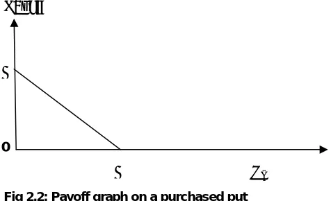
The second is to buy a put. That is, purchase an option to sell the underlying commodity or asset. Payoff on a purchased put= max[0, K-ST]. This is shown in Figure 2.2 below.

Payoff

Fig 2.2: Payoff graph on a purchased put

The third is to sell a call. That is write a contract that gives the purchaser the option to buy the underlying commodity or asset.

Payoff on a written call= -max[0, ST-K]. This is shown in Figure 2.3 below.

Payoff

0

K ST

Fig 2.3: Payoff graph on a written call

The fourth is to sell a put. That is, write a contract that gives the purchaser the option to sell the underlying commodity or asset.

Payoff on a written put= -max[0, K-ST]. This is shown in Figure 2.4 below.

Payoff

0

K ST -K

Fig 2.4: Payoff graph on a written put

The profit on a position= payoff on position-future

value of net cost on position.

Cost is positive when premium is paid in attaining the position and it’s negative when premium is received. Therefore, net cost can be positive or negative.

Volatility : Volatility is the most important factor in option pricing. It measures the likely magnitude of price changes over a given period, and is expressed as a percentage of the underlying market price. Volatility is calculated as the annualized standard deviation of the distribution of percentage changes in daily prices, which is assumed to be a normal distribution. The time value of an option increases 0

K ST

K

0

69 with the volatility of the market. If volatility is expected to be low, the future trading range will be narrower and the present value of the potential income stream from holding an option will be smaller since there is a lower probability of a large change in prices before expiry. However, if volatility is expected to be high, the future trading range will be wider and the present value of the potential income stream from holding an option will be larger since there is a higher probability of a large change in prices before expiry (Natenberg, 1994).

There are two types of price volatility used in pricing options. These are the Historical volatility and the Implied volatility.

Historical volatility – as its name suggests – is the range that prices have traded in over a given period in the past. Historical volatility allows us to see how prices have behaved under known market conditions. From this, we may be able to build a confidence level to help us in assessing the predictability of current situations. Volatility is defined in terms of variations in the proportionate change in price. Therefore, when finding an estimated value of it, we must take the standard deviation of ln(St/St-1). We observe these ratios daily, weekly or monthly and obtain an estimate of daily, weekly or monthly volatility. Then we multiply this by the square root of 365 over the unit (that is, 365 for days, 52 for weeks, 12 for months) to obtain the annual volatility (Weishaus, 2008).

Choosing an appropriate number of data to be used in the volatility estimation is not easy. More data generally lead to more accuracy, but volatility does change over time and data that are too old may not be relevant for predicting the future volatility. An often-used rule of thumb is to set the number of data equal to the number of days to which the volatility is to be applied. Thus, if the volatility estimate is to be used to value a 1-year option, data for the last year is used (Hull, 2006).

Implied volatility is the range that prices are expected to trade over a given period in the future. Implied values are calculated by inputting option premiums into an option pricing model.

Black-Scholes Pricing Model: In financial terms, the price of an option is simply the present value of the future income stream that can be expected from holding the option contract (Fusaro, 1998).

In the early 1970’s, Fischer Black, Myron Scholes and Robert Merton made a major breakthrough in the pricing of stock options. This involved the development of what has become known as the Black-Scholes model. The model has had a huge influence on the way that traders price and hedge options.

Assumptions

The Black-Scholes model is based on a few simplifying assumptions.

1. Stocks pay no dividends during the life of the option.

2. The Black-Scholes model only prices European call options.

3. No commissions are charged.

4. Interest rates and volatility remain constant and known.

5. Stock prices are lognormally distributed. 6. Markets are efficient.

7. Shares of a stock can be divided.

Brownian Motion

The Black-Scholes formula is a closed-form formula for evaluating the value of a European option. This pricing is based on the assumption that the movement of asset prices follows some sort of random walk. A (one-dimensional) discrete random walk models somebody starting out on the x-axis at the point 0 and then moving left or right at the rate of 1 per unit time, with the direction being chosen randomly. Suppose that instead of moving 1 per unit of time, we moved

h

_per

h

_{units of time and took} the limit as

h

→

0

. Then we would have a continuous random walk which is a normal random variable, and we would have Brownian motion. This is also known as the Wiener process (Weishaus, 2008).

Brownian motion Z t( )is a random process, a collection of variables indexed by time

t

, defined by the following properties:

1.

Z

(0)

=

0

2. Z t( )has a normal distribution with mean 0and variance

t

.

3. Increments are independent

4.

Z t

( )

is continuous in

t

.

70 process where only the present value of a variable is relevant for predicting the future. The third property of the Brownian motion stated above implies that Z t( )

follows a Markov process.

Arithmetic Brownian motion (or the generalized Weiner process) consists of a Brownian motion scaled by multiplication and shifted by addition. The mean change per unit time for a stochastic process is known as the drift rate and the variance per unit time is known as the variance rate. If X t( ) is an arithmetic Brownian motion (and note that

Z t

( )

is Brownian motion), then

X t( )=

α

t+

σ

Z t( )

Thus,X t( +s)−X t( ) has a normal distribution with mean

α

s

and variance 2

s

σ

.

α

is the expected drift rate per unit of time and

σ

is called the volatility of the process.

Arithmetic Brownian motion is not a good model for stock price movement because, it can go negative and does not scale with stock price; one would expect the proportional movement of stock price, rather than the arithmetic movement, to follow a constant distribution. Just like we transform a normal distribution to a lognormal distribution, we transform arithmetic Brownian motion to geometric Brownian motion.

To calculate the distribution of a geometric Brownian motionX u( ), let

t

be the latest time for which you have the value of X t( ). Then lnX t( +s s), >0, is

normally distributed with mean 2

ln

X t

( )

+

(

α

−

0.5

σ

)

s

and variance 2

s

σ

. For a stock with annual continuous return

α

and annual continuous dividend

δ

, the drift will be

α δ

−

. The value at time

t

of a geometric Brownian motion with drift

α

and volatility

σ

can be expressed as

2

ln

X t

( )

=

ln

X

(0)

+

(

α

−

0.5

σ

)

t

+

σ

Z t

( )

_(4.1)

The Black-Scholes Formula

From equation (4.1), if

S

_Tand

S

₀are the prices of the underlying security at time

T

and

0

respectively, then

2 0

ln

S

_T

=

ln

S

+

(

α

−

0.5

σ

)

T

+

σ

Z

In fact, it can be easily seen from the above equation that, the change in

ln

S

_{between time}

0

and some

future time

T

is normally distributed, with mean 2

(

α

−

0.5

σ

)

T

and variance

σ

2_{T . That is,}

2 2

0

ln

S

T

−

ln

S

~

N

⎣

⎡

(

α

−

0.5

σ

) ,

T

σ

T

⎤

⎦

or

2 2

0

ln

S

_T

~

N

_⎣

⎡

ln

S

+

(

α

−

0.5

σ

) ,

T

σ

T

⎤

_⎦

Which shows that

S

_T follows a lognormal distribution.

In a risk-neutral world,

α

is replaced with the continuous compound interest rate

r

.

The principle of risk-neutral valuation implies that the present value of the option is the expected final value of the option discounted at the risk-free interest rate. Let us consider a call option, which is known to have a final value of

max(

S

_T

−

K

, 0)

at time

T

. By the risk-neutral principle, the premium,

C

_{paid for this} option at time

0

is

[max(

, 0)]

(

) (

)

rT

T

rT

T T T

K

C

e

E

S

K

e

S

K f S dS

−

∞ −

=

−

=

∫

−

where

f S

(

T

)

, the probability density function of

T

S

(lognormal) can be explicitly written as

2 2

0

2

1

[ln

(ln

( 0.5 ) )]

1

₂

( )

exp

2

T T

T

S

S

r

T

f S

T

S

T

σ

σ

σ

π

⎛

₋

₋

_{+ −}

⎞

⎜

=

_⎜

⎜

⎝

⎠

2 2 0 2

1

[ln

(ln

( 0.5 ) )]

1

₂

(

)

exp

2

T rT T T K T

S

S

r

T

C e

S K

dS

T

S

T

σ

σ

σ

π

∞ −

⎛

₋

₋

_{+ −}

⎞

⎜

⎟

=

−

_⎜

_⎟

⎜

⎟

⎝

⎠

∫

Solving this integral, we get

C

=

S N d

₀

(

₁

)

−

Ke

−rT

N d

(

₂

)

(4.2) where 2 0 1

ln

2

,

S

r

T

K

d

T

σ

σ

⎛

⎞

⎛

_{⎞ + +}

⎜

⎟

⎜

⎟

⎝

⎠ ⎝

⎠

=

and _{2 1} 2 0

ln

2

S

r

T

K

d

d

T

71

( )

N x _{is the cumulative distribution for the standard}

normal distribution. In other contexts, N x( ) is known as Φ(x).

Equation (4.2) is the Black-Scholes formula for a call option on non-dividend stock.

The corresponding price for a put option on non-dividend stock is given by,

The general form of the Black-Scholes formula for a call option is

1 2

( )

(

)

(

)

(

)

P P

C

=

F

S N d

−

F

K N d

where

2

1

1

ln(

( ) /

(

))

2

P P

F

S

F

K

T

d

T

σ

σ

+

=

and

2

2 1

1

ln(

( ) /

(

))

2

P P

F

S

F

K

T

d

d

T

T

σ

σ

σ

−

=

=

−

In this equation, P

F

indicate a pre-paid forward price (present value of forward price).

S

is the underlying asset-that is the asset which you may elect to receive at the end of the period,

T

.

K

is the strike asset-which is the asset you may elect to pay at the end of the period,

T

. Data Analysis: The study was limited to secondary data obtained from The Energy Information

Administration on weekly all countries spot price of crude oil from January 2006 to October 2009. The Black-Scholes model is used for the computation of the options prices and some of the trading strategies of the options used in hedging commodities like crude oil are looked at.

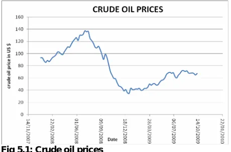
Figure 5.1 shows the fluctuations in crude oil prices over a period of two years (October 2007-October 2009).

Fig 5.1: Crude oil prices

Hedging with Options: Options can be used to achieve a great variety of possible outcomes depending on the exposure and risk preferences of the user. The next two sections describe common option trading strategies that are widely used in the oil industry.

Producer Hedge: An oil producer or distributor would like to hedge the value of its production. On October 9, 2009 (the day that the data was analyzed) the price of crude oil is $x/barrel. The producer expects prices to fluctuate during the two years period of the hedge (from October 9, 2009 – October 9, 20ll), but is concerned about the risk of prices falling below $y/barrel. If the producer is also prepared to accept a maximum price of $z/barrel for its production, a combination of put and call options can be used to hedge. Buy a $y/barrel put option and sell a $z/barrel call option. The result of this strategy is to limit the downside and upside price risks to a range between $y/barrel and $z/barrel.

If prices of crude oil fall below $y/barrel at the end of two years, the $z call option will be worthless but the $y put option will be exercised giving the producer the right to sell its output at $y/barrel, however low prices go. If prices rise above $z/barrel, the $y put option will be worthless, the $z call option will be exercised and the producer will be obliged to sell crude at $z/barrel, however high prices go. If prices are between $y/barrel and $z/barrel, neither of the options will be exercised and the producer sells its crude at the prevailing market price. This strategy is known as a collar. The strike price of the option can be set at any level, but the put and call options must be equally far out-of-the money if the cost of the put and call is to be the same. If the costs of the options are the same, the strategy is known as a zero cost collar (Cherry, 2007).

2 0 1

(

)

(

)

rT

72 Consumer Hedge: A crude oil consumer has based its crude oil purchasing plan on a maximum price of $x/barrel in two years time. In order to protect themselves against a price move above $x/barrel, the purchasing department could buy a two years $x call option. The result of this strategy is to limit the upside price risk so that the maximum price paid by the company for crude oil would be $x/barrel (Hull, 2006).

If prices rise above $x/barrel at the end of two years, the call option will be exercised and the company can obtain its supplies from the option writer at $x/barrel. However, if prices remain below $x/barrel, the $x call option will not be exercised and the purchasing department can meet its plan target with direct purchases on the spot market. However, the purchasing department will lose the premium paid at the beginning of the transaction (at time 0) for the call option. The combined profit on the crude oil and purchased call will then be equal to the profit on the purchased call.

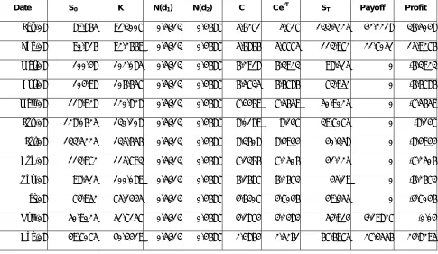
The values as shown in Table 1 and Table 2 indicate the profit that would have been realized if a consumer (or Ghana Government) had hedged crude oil prices in 2007 and 2008 respectively. The spot price for each month is the monthly average crude oil price (dollars per barrel) and the volatility is estimated from crude oil prices in the previous year. For the year 2007, the Volatility=0.1915 and for the year 2008, the Volatility=0.2222.

The expiration time is six months (T=0.5) and the strike price is the forward price of the monthly spot price (K=S0erT). In fact, these derivative traders usually use LIBOR (London Interbank Offer Rate) as short-term risk-free rates. This is because they regard LIBOR as their opportunity cost of capital. For the year 2007, Interest rate=0.0528 and for the year 2008, Interest rate=0.0317.

Table 1: Hedging in 2007

Date S0 K N(d1) N(d2) C CerT ST Payoff Profit

Jan-07 50.7725 52.1307 0.527 0.473 2.7407 2.814 72.8675 20.7368 17.9227 Feb-07 53.65 55.0852 0.527 0.473 2.896 2.9735 69.478 14.3928 11.4193

Mar-07 58.698 60.2683 0.527 0.473 3.1685 3.2533 73.8825 13.6142 10.361

Apr-07 63.6725 65.3758 0.527 0.473 3.437 3.529 78.155 12.7792 9.25018

May-07 63.905 65.6146 0.527 0.473 3.4496 3.5419 88.862 23.2474 19.7056

Jun-07 66.894 68.6835 0.527 0.473 3.6109 3.7075 87.62 18.9365 15.229

Jul-07 72.8675 74.8168 0.527 0.473 3.9334 4.0386 89.865 15.0482 11.0096

Aug-07 69.478 71.3366 0.527 0.473 3.7504 3.8507 90.816 19.4794 15.6286

Sep-07 73.8825 75.859 0.527 0.473 3.9882 4.0949 100.48 24.621 20.5262

Oct-07 78.155 80.2458 0.527 0.473 4.2188 4.3317 104.98 24.7342 20.4026

Nov-07 88.862 91.2392 0.527 0.473 4.7968 4.9251 118.928 27.6888 22.7637

Dec-07 87.62 89.964 0.527 0.473 4.7297 4.8562 128.063 38.0985 33.2423

73 Table 2: Hedging in 2008

Date S0 K N(d1) N(d2) C CerT ST Payoff Profit

Jan-08 89.865 91.3007 0.5313 0.4687 5.6271 5.717 133.5225 42.2218 36.5048

Feb-08 90.816 92.2669 0.5313 0.4687 5.6866 5.7775 113.972 21.7051 15.9276

Mar-08 100.48 102.085 0.5313 0.4687 6.2918 6.3923 98.515 0 -6.3923

Apr-08 104.98 106.657 0.5313 0.4687 6.5735 6.6786 73.952 0 -6.6786

May-08 118.928 120.828 0.5313 0.4687 7.4469 7.5659 50.9025 0 -7.5659

Jun-08 128.0625 130.108 0.5313 0.4687 8.0189 8.147 39.7075 0 -8.147

Jul-08 133.5225 135.656 0.5313 0.4687 8.3608 8.4944 40.358 0 -8.4944

Aug-08 113.972 115.793 0.5313 0.4687 7.1366 7.2506 41.225 0 -7.2506

Sep-08 98.515 100.089 0.5313 0.4687 6.1687 6.2673 45.19 0 -6.2673

Oct-08 73.952 75.1335 0.5313 0.4687 4.6307 4.7046 49.355 0 -4.7046

Nov-08 50.9025 51.7157 0.5313 0.4687 3.1874 3.2383 54.914 3.19827 -0.04

Dec-08 39.7075 40.3419 0.5313 0.4687 2.4864 2.5261 67.6975 27.3556 24.8295

Total profit=$21.72133

The total gain and total loss for 2007 and 2008 are illustrated in Figure 5.2 below.

Fig 5.2: Graph of total gain and total loss

Analysis and Discussion of results: Options enable companies to lock in a maximum or minimum

price for the purchase or sale of oil at a future date in exchange for a fixed non-refundable “insurance” premium. When options are used in hedging, the losses are limited to the premium paid.

The Black-Scholes model is used for pricing European options and some of the factors that affect the price of options are the current stock price, the strike price, the time to expiration, risk-free rate and the volatility. Currently, the price of crude oil has become very volatile with an estimated annual volatility of 42.69%. From Table 1, no losses were observed in the year 2007 as a result of hedging and even though some losses were recorded in the year 2008 (from Table 2), the profit recorded was positive.

Standard deviation is the measure of dispersion of a set of data from its mean and according to the Black-Scholes model, stock prices have standard deviation of

σ

T

.

74 CONCLUSIONS:

The above analysis shows that, it is prudent and financially beneficial for the government of Ghana to go into hedging using short maturity options. Hedging stabilizes the fluctuations of company’s cash flows. Hedging decreases company’s price risk exposure when being involved with physical products. It also provides effective financial management of the company and enables management to focus on other factors of the business. Also, options are more flexible compared to other derivative instruments used in price risk management. Short maturity options are cheaper and with less risk as compared to long maturity options and hedging with options secure competitive advantage by locking in high/low prices.

REFERENCES

[1] Cherry, H. (2007). Financial Economics, first edition. Actuarial Study Materials, 3217 Wynsum Ave., Merrick, NY 11566.

[2] Energy Information Administration. Weekly all countries spot price of crude oil.

http://tonto.eia.doe.gov/dnav/pet/hist/wtotopecw.htm, (accessed 2009 October 10)

[3] Fusaro, P.C. (1998). Energy Risk Management: Hedging Strategies and Instruments for the International Energy Markets, first edition. New York: McGraw-Hill. pp. 9-37

[4] Hull, C. J., (2006). Options, futures and Other Derivatives, sixth edition. Pearson Prentice Hall. pp. 99-373

[5] Long, D., (2000) Oil Trading Manual, Cambridge: Woodhead Publishing Ltd., Supplement 3.

[6] McDonald, L.R. (2006). Derivatives Market, second edition. Pearson Education, Inc.

[7] Natenberg, S., (1994), Option Volatility & Pricing: Advanced Trading Strategies and Techniques, Chicago: Probus Publishing Company. pp. 257-330.