Modeling of the Maximum Entropy Problem as an Optimal
Control Problem and its Application to pdf Estimation of
Electricity Price
M. E. Hajiabadi* and H. Rajabi Mashhadi**
Abstract: This paper proposes a novel two step modeling and analysis on the continuous random variable of electricity price. At the first step, the continuous optimal control theory is used to model and solve the maximum entropy problem for a continuous random variable. The maximum entropy principle provides a method to obtain least-biased Probability Density Function (pdf) estimation. In this paper, to find a closed form solution for the maximum entropy problem with any number of moment constraints, the entropy is considered as a functional measure and the moment constraints are considered as the state equations. Therefore, the pdf estimation problem can be reformulated as the optimal control problem. At the second step, the proposed unbiased pdf estimator is used to estimate the pdf of electricity price. Moreover, the statistical indices and the distributional characteristics of electricity price are analyzed at each load level. The simulation results on the electricity price data of New England, Ontario and Nord Pool electricity markets show the efficiency of the proposed pdf estimator. In addition, the obtained results show that by decreasing the load, the statistical and distributional characteristics of the electricity price inclined toward the statistical properties of the normal distribution.
Keywords: Electricity price, Maximum entropy (ME), Optimal control, Probability density function (pdf).
1 Introduction1
1.1 Motivation
In a restructured electricity market, electricity price is the most important signal for all market participants [1] and has different statistical characteristics compared to other markets. Therefore, several studies have been presented specifically on electricity price analysis and modeling. In [2-4] classifications of the considered methods and tools in electricity price modeling are presented.
Generally, analyses on electricity price are aimed at two different goals. The first goal is to present a forecasting model for the price and its volatility. Important tools applied in this area are such as Time series method, neural networks, wavelet transform,
Iranian Journal of Electrical & Electronic Engineering, 2013. Paper first received 20 Jun. 2012 and in revised form 5 Jan. 2013. * The Author is with the Department of Electrical Engineering, Ferdowsi University of Mashhad, Mashhad, Iran.
** The Author is with the Department of Electrical Engineering at Ferdowsi University of Mashhad and the Center of Excellence on Soft Computing and Intelligent Information Processing, Ferdowsi University of Mashhad, Mashhad, Iran.
E-mails: [email protected] and [email protected].
fuzzy logic, Weighted Nearest Neighbors (WNN) techniques and hybrid methods. The second goal is to get a good understanding of the electricity price behavior and electricity market operation using statistical and probabilistic approaches. Results that achieved by these analyses can affect the player's strategies and thus economic benefits of them [5]. Moreover, through a right understanding of the electricity price behavior, the market regulator is able to monitor the level of the competitiveness of the market [6].
1.2 Literature Review 1.2.1 Study the pdf of Electricity Price
Application of the electricity price pdf to risk management, evaluating the risk associated with the deviation of actual prices from a particular forecast, options valuation, etc is indispensable [1]. Moreover, the probability distribution of price is used in short-term, [4, 7, 8], mid-short-term, [9, 10] and long-term [11] modeling and forecasting of the electricity price. Analysis of the pdf of electricity price at different market conditions plays the role of a monitoring tool for the market operator [6]. The relationship between the
system surplus capacities percent and price pdf has been indicated in [6]. It's statistically shown that at high load, which the supply and demand relationship becomes intense, the distribution of price deviates from the normal distribution. Proposing an efficient analytic method for assigning a pdf to the random variable of the electricity price has become the center of attention of many researchers. The calculation of electricity price pdf with two methods has been discussed in [1]: statistical method and Artificial Neural Network (ANN). In [12] Inverse-Quantile function has been used to fit two special classes of distributions to electricity price. Panagiotelis and Smith in [13], applied multivariate skew t distribution to estimate the pdf of electricity price. An analytical relationship between the system load level, the structure of price formation and the distribution of Locational Marginal Price (LMP) from the planning viewpoint has been proposed in [14].
1.2.2 Entropy and Electricity Market
Entropy is a measure of uncertainty associated with the random variable. It defines the expected value of the random variable information [15]. This concept has been applied for data mining in the field of electricity market price forecasting in [16]. The entropy coefficient is used as a measure of market concentration in [17, 18]. Permutation entropy, topological entropy and the modified permutation entropy are used as the measures of volatility in electricity markets in [19]. The electricity purchase risk is mainly related to the uncertainties of electricity price. In other words risk is arisen from market change or some uncertain events in the future. This means that the risk and entropy have the same essence [20]. In [20] the information entropy has been introduced as risk measure for electricity purchase.
1.2.3 Optimal Control Theory
Optimal control theory is used to find an optimal solution in controlling a dynamic system. It models a process and its constraints as state equations and finds a control law (optimal control policy) for a given system such that a certain optimality criterion is achieved. Starting point to study a process with optimal control is to model the process as a set of differential equations (state space equations) [21, 22]. Optimal control has numerous applications in design of the marine systems, aerospace, robots, industrial processes, power systems, energy management, economic systems, bio-medical models and control of environment systems [21, 23].
1.3 Contributions
This paper proposes a novel two step modeling and analysis on the continuous random variable of electricity price. At the first step, the problem of the pdf estimation of electricity price is analyzed in viewpoint of information theory. The concept of maximizing the information of a random variable has resulted in the use of the maximum entropy method which provides a mean
to obtain least-biased pdf estimator [19]. The maximum entropy problem for a continuous random variable, such as electricity price, introduces a functional optimization problem. Thus, in this paper the structure of optimal control problem is utilized to model entropy maximization problem for continuous random variable. Hence, the entropy is considered as a functional and relevant moment constraints are modeled as the state space equations. One of the noteworthy advantages of the proposed approach is the possibility to easily consider any quantity of moment constraints and to reach a closed form solution for the probably density function using optimal control theory. Moreover, modeling the entropy maximization as a state space and an optimal control problem can be itself very beneficial in other researches.
At the second step, the proposed unbiased pdf estimator is used to estimate the probability density functions of the electricity price. Moreover, the statistical indices and the distributional characteristics of electricity price are analyzed at each load level. As shown in Fig. 1, the main goal of these analyses is to provide a relation betwean the electricity price and the electricity market operation.
The simulation results on the electricity price data of New England, Ontario and Nord Pool electricity markets show the efficiency of the proposed pdf estimator. The pdf estimation is done for the electricity price at three different load levels. Moreover, by using the quantitative and qualitative methods, the statistical properties of electricity price are analyzed at each load level. The obtained results show that by decreasing the load, the statistical and distributional characteristics of the electricity price inclined toward the statistical properties of the normal distribution.
1.4 Paper Organization
This paper is organized as follow: the maximum entropy and the optimal control problems are introduced in section 2. The maximum entropy problem is modeled as the optimal control problem in section 3. Section 4 introduces the proposed unbiased pdf estimator for the continuse random variable. Section 5 includes the simulation results of pdf estimation of electricity price. Finally, the paper is summarized and concluded in section 6.
Fig. 1 Market operation and electricity price.
2 Problem Formulation
2.1 Entropy and Maximum Entropy
Entropy of a random variable X, defined by H(X), is a measure of the uncertainty associated with the random variable. Shannon quantifies the entropy of X as the expected value of its information (I). The entropy of discrete random variable X is expressed by:
1 1
( ) ( ) ln
n n
i i i i
i i
H X E I pr I pr pr
= =
= =
∑
× = −∑
× (1)If X be a continuous random variable, e.g. electricity price signal, the entropy is defined similarly as:
max max
min min
1
( ) ( ) ln ( ) ln ( )
( )
x x
x x
H X f x dx f x f x dx
f x
=
∫
= −∫
(2)where, f(x) is the pdf of the random variable X and (xmin , xmax) is the range of variation of X [15].
Maximum entropy method tries to choose a proper probability density function for a random variable based on its statistical moments, such that the maximum information from the data is obtained [15]. In this method, the moment constraints guaranty that the estimated probability distribution is identical to the experimental data. Moreover, considering the concept of information maximization, this method applies minimum presumptions of random variables for estimation of its pdf. In other words, the main advantage of the maximum entropy is to provide a method to obtain least-biased pdf estimation. Hence, it makes sense to term the maximum entropy method for the estimation of the probability density function as an
Unbiased pdf Estimator. Eq. (3) shows the problem of entropy maximization for a continuous random variable, under the natural constraint and the first m moment constraints.
max
min max
min
( )
1
( ) ln ( ) ln ( )
( )
( ) 1
:
( ) 1, 2,...,
f x
x x x
r
r x
Max H f x dx f x f x dx
f x
f x dx
such that
x f x dx a r m
= = −
⎧
⎪ =
⎪ ⎪ ⎨ ⎪
= =
⎪ ⎪⎩
∫
∫
∫
∫
(3)
where ar for r = 1, 2…, m are the constant moment
values.
2.2 Optimal Control Problem and the Necessary Conditions for the Optimality
Optimal control is developed to find the optimal control input u* for a system with state space representation A in Eq. (4), such that the system takes the optimal trajectory y* in a way that the performance measure J is minimized [22].
0
( ) ( ( ), ( ), )
( ( ), ) ( ( ), ( ), )
f t
f f
t y t A y t u t t
J h y t t g y t u t t d t
=
= +
∫
&
(4)
where, t0 and tf are the initial and the final times and h
and g are the scalar functions. To find optimal control input u*, at first the Hamiltonian function is formed and then the necessary conditions for optimization are observed:
(
)
* * *
* * *
* * *
( , , , ) ( , , ) [ ( , , )]
( ) ( ( ) , ( ) , ( ) , )
( ) ( ( ) , ( ) , ( ) , )
0 ( ) , ( ) , ( ) ,
T
Ham ilt y u p t g y u t p A y u t
Ham ilt
y t y t u t p t t
p Ham ilt
p t y t u t p t t
y Ham ilt
y t u t p t t
u •
•
= +
∂ =
∂ ∂ = −
∂ ∂ =
∂
(5)
where p(t) is the Lagrange multipliers vector related to co-state equations.
3 Modeling the Maximum Entropy as an Optimal Control Problem and its Solution
Maximum entropy problem for a continuous random variable such as electricity price introduces a functional optimization. Thus in this section, the Lemma 1 is introduced and proved to model the maximum entropy problem for a continuous random variable as an optimal control problem. Therefore, the entropy is considered as a functional and the moment constraints as the state space equations.
3.1 Modeling the Maximum Entropy as an Optimal Control Problem
By assuming that the x, xminand xmax in Eq. (3) are
equal with t, t0and tf in optimal control problem in Eq.
(4), respectively, and also the decision variable f(x) equals with the control input u(t), then the following lemma is introduced.
Lemma 1:
The maximum entropy problem for a continuous random variable with m moment constraints is equivalent by the optimal control problem with state space representation in Eq. (6) and the performance measure in Eq. (7).
( ) ( )
( ) ( ( ), ( ), )
( )
m
u t tu t y t A y t u t t
t u t •
⎡ ⎤
⎢ ⎥
⎢ ⎥
= = ⎢ ⎥
⎢ ⎥
⎢ ⎥
⎣ ⎦
M (6)
0
( ) ln( ( )) f
t
t
J =
∫
u t u t dt (7)Proof:
Eq. (8) shows that the natural constraint in Eq. (3) could be rewritten as the state space equation with known final condition.
max 0 min 0 max min 1 ( ) ( ) 1 1 ( ) ( )
( ) 1
( ) 1
( ) ( )
( ) 1
f t x
f x u t t x t x t x f f
u d y t
f x dx
y t y t u t y t = = = • ⎧ = ⎪ = ⎯⎯⎯⎯→ ⎨ ⎪ = ⎩ ⎧⎪ = → ⎨ = ⎪⎩
∫
∫
τ τ(8)
Simultaneously, the moment constraints can be transformed. Eq. (9) shows the state space equations which are equivalent by the moment constraints:
max 0 m in ( ) ( ) ( ) ( ) ( ) ( ) 1, ..., ( ) t r x r r t r x
r f r
r r
f r
u d y t
x f x dx a
y t a
y t t u t r m
y t a
• ⎧ = ⎪ = → ⎨ ⎪ = ⎩ ⎧⎪ = → ⎨ ∀ = = ⎪⎩
∫
∫
τ τ τ(9)
The state space model in Eq. (6) is obtained from the Eqs. (8) and (9). Moreover, the maximization problem in Eq. (3) can be replaced by the minimization problem in Eq. (10).
m a x
m in
0 m in m a x
0
( )
( ) ( ) &
( )
( ) ln ( )
m in ( ) ln ( ( ))
f f x f x
x u t f x t x t x
t u t
t
M a x H f x f x d x
J u t u t d t
= = = = − =
∫
∫
c
c
(10)Therefore, the performance measure in Eq. (7) is obtained from the Eq. (10) and the Lemma 1 is proved.
3.2 Solution of the Equivalent Optimal Control Problem
To find the optimal control input u*(t) for the system with state space representation in Eq. (6), such that J in Eq. (7) is minimized, first the Hamiltonian function is formed. The Hamilton function related to the equivalent optimal control problem is expressed in Eq. (11).
1 2 1 ( ) ( ) ( ) ( )
( ( ), ( ), ( ), ) ( )ln( ( ))
( ) ( ) T m m u t p t tu t p t
Hamilt y t u t p t t u t u t
p + t t u t
⎡ ⎤ ⎡ ⎤ ⎢ ⎥ ⎢ ⎥ ⎢ ⎥ ⎢ ⎥ = +⎢ ⎥ ⎢ ⎥ ⎢ ⎥ ⎢ ⎥ ⎢ ⎥ ⎣ ⎦ ⎣ ⎦ M M (11)
The necessary conditions for the optimality are presented in Eq. (12). The second necessary condition is the co-state equations. According to Eq. (11), the Hamiltonian function is independent from the state variable y. Therefore, as indicated in Eq. (12), the Lagrange multipliers pi are constant values. By solving
the third necessary condition and considering constant
values for the pi, the optimal control input u*(t) is
obtained.
(
)
* * * * *
* * *
* * *
1 2 1
( ) ( ( ) , ( ) , ( ) , ) ( ( ) , ( ) , )
( ) ( ( ) , ( ) , ( ) , ) 0 ( )
0 ( ) , ( ) , ( ) ,
ln( ( )) 1 ... r m 0
Hamilt
y t y t u t p t t A y t u t t
p Hamilt
p t y t u t p t t p t cons
y Hamilt
y t u t p t t
u
u t p tp t p
• • + ∂ = = ∂ ∂ = − = ⇒ = ∂ ∂ = ∂ ⇒ + + + + + = (12)
Therefore, the optimal control input u*(t) can be expressed as Eq. (13).
1 2 1
( ) exp( (1 ... m m ))
u t = − +p +tp + +t p + (13)
In Eq. (13) the m+1 Lagrange multipliers pi are
constant values and unknown parameters. These parameters are calculated by using the final conditions in Eqs. (8) and (9). Therefore, the Lagrange multipliers
pis are obtained by solving the m+1 simultaneous
equations in Eq. (14):
0
0
( ) 1
( ) 1, 2 , ...,
f f t t t r r t
u t d t
t u t d t a r m
=
= ∀ =
∫
∫
(14)
Because of the complexity of these simultaneous equations, heuristic methods such as genetic algorithm are used to solve the equations.
4 Unbiased pdf Estimation of a Continues Random Variable
As mentioned in section 2, the maximum entropy method can be used as an Unbiased pdf Estimator. In Lemma 1 it was proved that the maximum entropy problem can be reformulated as an optimal control problem. Eqs. (13) and (14) show the solution of this optimal control problem. Based on the proposed method, the following process is presented as an Unbiased pdf Estimator. This process assigns an unbiased probability density function to a continuous random variable (especially electricity price):
1. Omitting the improper data from the existing data of the continuous random variable; 2. Calculating the first statistical moments (ar)
from the modified data;
3. Solving the simultaneous in Eq. (14) and calculating the Lagrange coefficients (pi).
4. Assigning the unbiased probability density function f(x) = exp(-(1+p1+xp2+...+xpm+1)) to the continuous random variable X. This function is assigned on the interval (xmin , xmax). 5 Pdf Estimation of Electricity Price and Electricity Market Analysis
One of the main goals of this paper is to estimate the probability distribution of the electricity price and
analysis of the statistical indices and the distributional characteristics of electricity price at the different load levels. Therefore, the proposed nonparametric method, which is an unbiased pdf estimator, is used to estimate the pdf of electricity price. The first four statistical moments e.g. mean, variance, skewness and kurtosis are used as the moment constraints. Skewness and kurtosis are the measures of the "asymmetry" and "peakedness" of the probability distribution of a real-valued random variable respectively. Generally, to analyze the behavior and distributional characteristics of a random variable, the first four moments are used. In [24], it is mentioned that the first four statistical moments are the characterizing moments and the 5th moment and above have no essential affect on the distribution function. Therefore, the proposed unbiased pdf estimator gives
p1,..., p5.
5.1 Statistical Study
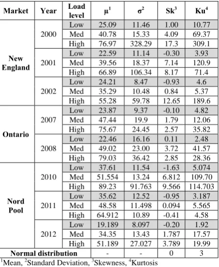
The load and price data in the New England, Ontario and Nord Pool electricity markets are used for the statistical study [25-27]. Table 1 shows the results of the statistical study on the electricity price in the considered markets at three load levels. The load levels are the low, median and high load levels. The high load data are the loads that higher than µl + σl, in which µl is the mean
load and σl is the standard deviation of the load. The low
load data are the loads that lower than µl- σl. Other load
data are considered as the median load data. As shown in this table, the skewness and kurtosis of the electricity
price are close to the statistical moments of the normal distribution at low load level (sk=0 and ku=3).
At high load, the price spikes influence the statistical properties of electricity price. Price spikes usually occur at high load and on specific market and network operational conditions. Therefore, price spikes are eliminated from the price data and then the electricity price data are analyzed at each load level. Afterwards the pdf of electricity price at each load level are estimated by using the unbiased pdf estimator, which was proposed in the previous section.
5.2 Unbiased pdf Estimation of Electricity Price
In this subsection, based on the four step process which proposed in section 5, an unbiased pdf is estimated and assigned for the random variable of electricity price at each load level. Table 1 shows the first four moment of electricity price at each load level. By solving the simultaneous in Eq. (14), the Lagrange coefficients p1,..., p5 are calculated. Table 2 shows the values of p1,..., p5 for the random variable of electricity price at each market, at each year and at each load level. As noted, these functions are defined in the interval of minimum up to maximum price for each load level.
Table 3 shows the closed form of the unbiased pdf of electricity price at each load level in the New England electricity market at year 2000. As illustrated in this table, the close forms of the pdf are derived based on the Lagrange coefficients which calculated in Table 2. These functions are plotted in Fig. 2.
The proposed unbiased pdf estimator is actually a nonparametric method. Hence, it is expected that the Table 1 Statistical study of price in the New England, Ontario
& Nord Pool electricity markets.
Market Year Load level µ1 σ2 Sk3 Ku4
New England
2000
Low 25.09 11.46 1.00 10.77 Med 40.78 15.33 4.09 69.37 High 76.97 328.29 17.3 309.1 2001
Low 22.59 11.14 -0.30 3.93 Med 39.56 18.37 7.14 120.9 High 66.89 106.34 8.17 71.4 2002
Low 24.21 8.47 -0.93 4.6 Med 35.29 10.48 0.84 5.37 High 55.28 59.78 12.65 189.6
Ontario
2007
Low 23.87 9.37 -0.10 4.82 Med 47.44 19.9 1.79 12.06 High 75.67 24.45 2.57 35.82 2008
Low 22.46 16.16 0.11 2.48 Med 49.02 23.00 3.72 41.57 High 79.03 36.42 2.85 28.36
Nord Pool
2010
Low 37.61 11.54 -1.63 5.074 Med 51.554 13.24 6.812 109.70 High 89.23 91.763 9.566 114.703 2011
Low 35.62 12.52 -0.95 3.187 Med 48.58 11.498 0.094 5.565 High 64.912 10.89 -0.41 4.58 2012
Low 19.189 8.097 -0.20 1.92 Med 34.35 13.43 1.787 17.57 High 51.189 27.027 3.789 19.99
Normal distribution - - 0 3
1
Mean, 2Standard Deviation, 3Skewness, 4Kurtosis
Table 2 Lagrange coefficients of price in the New England, Ontario & Nord Pool electricity markets.
Market YearLoad level p1 p2 p3 p4 p5 Price interval($/MWh)
New England
2000
Low -0.03 -5.91 2.72 0.76 8.10 (-2.6, 63.6) Med -0.36 -6.63 0.39 8.55 18.45 (2.2, 120.4) High -1.49 -1.66 1.95 3.15 6.5 (17.8, 128) 2001
Low 0.20 -8.98 4.80 7.75 7.17 (-6.45, 72.31) Med -0.35 -6.89 1.02 7.81 19.82 (0, 119.9) High -1.2 -2.05 0.08 3.81 6.34 (20.38, 120) 2002
Low 1.94 -9.48 0.15 2.28 9.73 (-5.96, 50.6) Med 0.31 -10.2 3.56 11.96 14.77 (0, 102.4) High -0.64 -6.27 7.01 4.52 1.79 (19.17, 106.4)
Ontario
2007
Low -0.54 -5.57 0.06 8.30 13.91 (-0.4, 73.94) Med -0.95 -4.09 1.7 5.62 9.48 (4.8, 142.3) High -0.64 -2.80 -1.16 3.82 4.98 (30.58,141.09) 2008
Low 1.38 -8.46 -1.72 4.01 12.58 (-34, 83.01) Med -0.33 -6.21 0.99 5.85 14.89 (-2.62, 146.1) High -1.21 0.25 -1.66 0.028 3.92 (26.31,146.29)
Nord Pool
2010
Low 1.81 -5.38 -5.24 4.15 5.30 (0.28, 59.58) Med -0.19 -10.1 9.06 8.17 14.94 (8.33, 148.01) High -1.8 0.07 3.44 -0.76 1.90 (40.16,169.25) 2011
Low 1.04 -4.48 -2.53 5.63 -0.58 (0.36, 55.44) Med -0.27 -7.46 0.5165 10.5 21.12 (3.49, 143.97) High 0.07 -6.39 2.41 -1.34 14.43 (36.47,106.89) 2012
Low -0.69 -1.12 -0.87 -1.15 4.58 (3.92, 36.23) Med -1.06 -4.16 2.27 4.24 15.66 (6.33, 103.48) High -2.23 2.21 2.43 -1.10 2.50 (28.8, 105)
estimated distribution function be more similar to the actual price distribution compared with the other parametric pdf estimators. For instance, in Fig. 3, the histogram of electricity price at high load level is compared with its estimated probability density functions. This figure graphically shows the efficiency of the proposed unbiased pdf estimator compared with Weibull and Extreme Value pdf estimators.
5.3 Electricity Market Analysis
As mentioned in section 1, one of the main goals of this paper is to analyze the statistical behaviors and the distributional characteristics of electricity price at various conditions of the load. In order to achieve this goal, the quantitative and qualitative analyses are used in this subsection.
5.3.1 Quantitative Comparison
The skewness, kurtosis and relative entropy of electricity price are used to quantitative comparison of price at each load level. As illustrated in Table 1 by increasing network load the electricity price skewness moves to the right and kurtosis level elevates. Hence when load increases in these networks, the electricity price pdf deviates from the normal distribution. The relative entropy can be used for the better comparison. Relative entropy is a measure of distance between two distributions. The relative entropy of distribution f and normal distribution φ is defined as bellow [15]:
( )
( ) ( )
( ) f x
D f x log dx
x
ϕ +∞
−∞
=
∫
× (15)Indeed, the decrease of the relative entropy to zero is equivalent to the convergence of distribution f to the normal distribution. Table 4 shows the relative entropy of electricity price at low and high load level. As shown in Table 4 by increasing the load the relative entropy of electricity price increases. Hence, when the load increases in these markets, the electricity price pdf deviates from the normal distribution.
5.3.2 Qualitative Comparison
Fig. 4 shows the pdf of electricity price at each load level in New England electricity market in 2000. Furthermore, the normal distributions related to each pdf are shown in this figure. As shown in Fig. 4, by increase of the system load the price distribution deviates from the normal distribution.
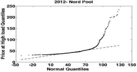
Figures 5 and 6 show the q-q plots of electricity price at high and low system load at Nord Pool electricity market at 2012, to compare the probability distributions of them by normal distribution.
The quantile-quantile plot, or q-q plot, is the graphical testing of the equality of two distributions. As shown in Fig. 5, the probability distribution of electricity price at off-peak system load similar to the normal distribution. However, Fig. 6 illustrates that at peak system load, the probability distribution of electricity price is different from the normal distribution.
Table 4 Relative entropy of price in the New England, Ontario & Nord Pool electricity markets.
R. E.1
Year Market
High Low
5.62 1.15
2001
New England
5.93 0.63
2002
4.92 1.98
2007
Ontario
4.28 0.59
2008
5.97 1.11
2010
Nord Pool 2011 0.8 0.76
3.73 0.92
2012
0
Normal pdf
1Relative Entropy with normal distribution Fig. 2 Unbiased pdf of electricity price at New England
electricity market, year 2000.
Fig. 3 Comparison of the histogram of electricity price with its estimated probability density functions.
Table 3 Unbiased pdf of electricity price in the New England electricity market at year 2000.
Load Closed form of pdf of electricity price Price interval
Low 2 3 4
(1 0.03 5.91 2.72 0.76 8.10 ) ( ) x x x x
f x =e− − − + + + (-2.6, 63.6)
Mid 2 3 4
(1 0.36 6.63 0.39 8.55 18.45 ) ( ) x x x x
f x =e− − − + + + (2.2, 120.4)
High 2 3 4
(1 1.49 1.66 1.95 3.15 6.5 ) ( ) x x x x
f x =e− − − + + + (17.8, 128)
6 Conclusion
The main goal of this paper was to provide a novel two step modeling and analysis on the continuous random variable of electricity price. For this purpose, at the first step the continuous optimal control theory was used to model and solve the maximum entropy problem for a continuous random variable. The maximum entropy principle provides a method to obtain least-biased pdf estimation. In the proposed method, the entropy was considered as a functional measure and the moment constraints were modeled as the state equations to find a closed form solution for the maximum entropy problem with any number of moment constraints. Therefore, the least-biased pdf estimation problem was formulated as an optimal control problem. At the second step, the proposed unbiased pdf estimator was used to
estimate the pdf of electricity price. Moreover, the statistical indices and the distributional characteristics of electricity price were analyzed at each load level. The simulation results on the electricity price data of New England, Ontario and Nord Pool electricity markets showed the efficiency of the proposed pdf estimator. The obtained results showed that by decreasing the load, the statistical and distributional characteristics of the electricity price inclined toward the statistical properties of the normal distribution.
References
[1] Shahidehpour M., Yamin H. and Li Z., Market
Operations in Electric Power Systems: Forecasting, Scheduling, and Risk Management, John Wiley & Sons. New York, 2002.
[2] Gonzalez A. M., Roque A. M. S. and Garcia-Gonzalez J., “Modeling and forecasting electricity prices with input/output hidden markov models”, IEEE Trans. Power systems, Vol. 20, No. 1, pp. 13-24, Feb. 2005.
[3] Li G., Liu C. C., Lawarree J., Gallanti M. and Venturini A., “State-of-the-art of electricity price forecasting”, in Proc. 2nd CIGRE/IEEE Power
Eng. Soc. Int. Symp, San Antonio, TX, pp.110-119, Oct. 2005.
[4] Vahidinasab V., Jadid S. and Kazemi A., “Day-ahead price forecasting in restructured power systems using artificial neural networks”, Electric
Power Systems Research, Vol. 78, No. 8, pp. 1332-1342, Aug. 2008.
[5] Barforoushi T., Moghaddam M. P., Javidi M. H. and Sheik-El-Eslami M. K., “A New Model Considering Uncertainties for Power Market Simulation in Medium-Term Generation Planning”, Iranian Journal of Electrical &
Electronic Engineering, Vol. 2, No. 2, pp. 71-81. Apr. 2006.
[6] Zhou H., Chen B., Han Z. X. and Zhang F. Q., “Study on probability distribution of prices in electricity market: A case study of Zhejiang province, China”, Commun Nonlinear Sci Numer
Simulat. No. 14, pp. 2255-2265, June 2008. [7] Zhao J. H., Dong Z. Y., Xu Z. and Wong K. P.,
“A statistical approach for interval forecasting of the electricity price”, IEEE Trans. on Power
systems, Vol. 23, No. 2, pp. 267-276, May 2008. [8] Weron R. and Misiorek A., “Forecasting spot
electricity prices: A comparison of parametric and semiparametric time series models”, International
Journal of Forecasting, Vol. 24, pp. 744-763, 2008.
[9] Davison M., Anderson C. L., Marcus B. and Anderson K., “Development of a hybrid model for electrical power spot prices”, IEEE Trans. on
Power systems, Vol. 17, No. 2, pp. 257-264, May 2002.
Fig. 4 Comparison of the estimated distribution functions of price with normal distribution.
Fig. 5 q-q plot: Compares the probability distribution of price at low load level with normal distribution.
Fig. 6 q-q plot: Compares the probability distribution of price at high load level with normal distribution.
[10] Ander system prices: outage
system
[11] Abdi H “A P Expan System
Electri
3, pp. 4 [12] Deng Functi Price” System [13] Panagi foreca multiv Journa 2008. [14] Bo R.
consid Power Aug. 2 [15] Cover Inform Sons, [16] Amjad Electri Netwo 21, No [17] Alvara reactiv Power pp. 294 [18] Kumar Electri Conve
[19] Ruiz M New A Marke [20] Zheng entrop electri
Society
[21] Sethi S
Theory Econo
son C. L. a m-econometric : considering e distribution
ms, Vol. 23, No H., Parsa Mog Probabilistic nsion Plannin
ms under Unc
ical & Electro
43-52. July 20 S. J. and Jia ion Approach
, 35th Hawai
m Sciences, pp iotelis A. and sting of intr variate skew t
al of Foreca
and Li F., “P dering load u
r systems, Vo 2009.
T. M. and
mation Theory
1991. dy N.,
“Day-icity Markets ork”, IEEE Tr o. 1, pp. 887-8 ado F. L. and ve market pow
r Engineering
4-296, 1999. r David A. an icity Supply”
ersion, Vol. 16 M., Guillamó Approach to ets”, Entropy, g Y., Zhou M
y based fuz city purchasin
y General Me
S. D. and Tho
y: Application mics, Springe
and Davison c model for g spike sensi ns”, IEEE Tr o. 3, pp. 927-9 ghaddam M. a
Approach t ng in Dere ertainties”, Ir
onic Engineer
005.
ang W., “An h for Mode
ii Internationa
p. 794-800, Jan d Smith M., “B
aday electric t distribution
asting, No. 2 Probabilistic L uncertainty”, I ol. 24, No. 3,
Thomas J.
y, New York -Ahead Price s by a New
rans. on Pow
896, May 2006 d Overbye T wer”, in Proc
Society 1999
nd Wen F., “M ”, IEEE Tra 6, No. 4, pp. 3 ón A. and G Measure Vol Vol. 14, pp. 7 M. and Li G zzy optimiza ng portfolio”,
eeting, PES '09
ompson G. L.,
ns to Managem
er, 2005.
M., “A hyb electricity s itivity to for
rans. On Pow
937, Aug 2008 and Javidi M. to Transmiss egulated Pow
ranian Journa ring. Vol. 1, N
Inverse-Quan eling Electri
al Conference
n 2002. Bayesian den ity prices us s”, Internatio 24, pp. 710-7
LMP forecast
IEEE Trans.
, pp. 1279-12
A., Elements k, John Wiley
e Forecasting w Fuzzy Neu
wer Systems, V 6.
. J., “Measur
ceedings of IE 9 Winter Meeti
Market Powe
ans. on Ene
52-360, 2001 Gabaldón A.,
atility in Ene 74-91, 2012. G., “Informat ation model
Power & Ene 9, July 2009.
Optimal Con ment Science a
brid spot rced wer 8. H., sion wer al of No. ntile city e on nsity sing onal 727, ting on 289, s of y & g of ural Vol. ring EEE ing, r in ergy . “A ergy tion of ergy trol and [22 [23 [24 [25 [26 [27 Ma sys Ger at F Exc Pro His pla com
2] Kirk D. E
an Introdu
3] Geering H
Applicatio 4] Srikanth “Probabili MinMax Man and Feb 2000.
5] New En
Reports. A 6] Ontario e Available 7] Nord Poo Available
ashhad, Mashha stem economics
rmany, in 2002 Ferdowsi Unive cellence on So ocessing, Ferdo s research int anning, power
mputation.
E. and Jose S
uction, Dover H. D., Optima
ons, Springer, M., Kesava ity density fun
measure”, IE
Cybernetics, .
ngland electr Available: http electricity M : http://www.i ol electricity M
: http://www.n
Mohamma
born in Ne received University Zahedan, Ir from Shari Tehran, Ira engineering the Ph.D engineering ad, Iran. His ar s and power sys
Habib Ra Mashhad, I B.Sc. and from the Mashhad, b and the Departmen Engineerin Tehran, Ira Aachen U 2. He is as Profe ersity of Mashh oft Computing wsi University terests are po r system e
., Optimal Co publication In
l Control with
2007. an H. K. a
nction estimat
EEE Trnas.
Vol. 30, No.
ricity Marke p://www.iso-n Market Operat ieso.ca. Market Opera nordpoolspot.
ad Ebrahim H
eyshabour, Iran the B.Sc. of Sistan & ran, in 2005 an if University o an, in 2008, bo g. Currently, h D. degree g at Ferdowsi reas of interest stem reliability
ajabi Mashhad
Iran, in 1967. H M.Sc. degree Ferdowsi U both in electric
Ph.D. degre nt of Electrical ng of Tehra
an, under joint University of fessor of electric hadand is with g and Intelligen of Mashhad,M ower system economics, an
ontrol Theory
nc, 1989.
h Engineering
and Roe P., tion using the
On Systems,
1, pp. 77-83,
et Operation ne.com.
tion Reports.
ation Reports. .com.
Hajiabadi was n, in 1983. He degree from & Baluchestan, d M.Sc. degree of Technology, oth in electrical he is pursuing in electrical University of include power evaluation.
di was born in He received the es with honor University of cal engineering, ee from the and Computer n University, cooperation of f Technology, cal engineering h the Center of nt Information Mashhad, Iran. operation and nd biological y g , e , n . . s e m , e , l g l f r n e r f , e r , f , g f n d l