International Journal of Engineering
J o u r n a l H o m e p a g e : w w w . i j e . i r
Using Modified IPSO-SQP Algorithm to Solve Nonlinear Time Optimal Bang-bang
Control Problem
T. Taleshian, A. Ranjbar*, R. Ghaderi
Department of Control Engineering, Babol University of Technology, Babol, Iran
P A P E R I N F O
Paper history:
Received 05 October 2012
Accepted in revised form 18 April 2013
Keywords: MIPSO-SQP Algorithm Time Optimal Bang-Bang Control Nonlinear Systems
Intelligent algorithm Gradients-Based Algorithm
A B S T R A C T
In this paper, an intelligent-gradient based algorithm is proposed to solve time optimal bang-bang control problem. The proposed algorithm is a combination of an intelligent algorithm called improved particle swarm optimization algorithm (IPSO) in the first stage of optimization process together with a gradient-based algorithm called successive quadratic programming method (SQP) in the second stage. The proposed algorithm is called MIPSO-SQP algorithm which in essence is a modification of the previous IPSO-SQP algorithm (PIPSO-SQP). New steps in optimization process of the proposed MIPSO-SQP algorithm causes the algorithm to reach to global optimal solution regardless of any guess of the initial control input and/or the number of switching. Validity of results is verified through adding some arcs to present arcs. The proposed algorithm is successfully applied in time optimal bang-bang control of the Van Der Pol equations, Rayleigh system and F8 aircraft model. A comparison study is also performed to assess the performance of MIPSO-SQP with respect to Switching Time Optimal method (TOS), mathematical programming method and PIPSO-SQP algorithm. It is shown that MIPSO-SQP algorithm is more effective than these algorithms due to ability to find global optimum solution in less iteration and in a more systematic way
doi:10.5829/idosi.ije.2013.26.11b.06
1. INTRODUCTION1
A wide variety of optimal control problems involves with mechanical dynamics in which the control input is switched between a lower and upper bound. This is called a two-position or bang-bang control, which is a good candidate to control such a physical system with limitations on its actuators. A wide variety of optimal control problems where the system is linear with respect to control input is of bang-bang type, for example On-Off mode of a thermostat [1]. However, one may deal with the bang-bang solution in other optimal control problems. This situation will especially occur in case where the Hamiltonian is linear with respect to control input especially when the solution is not singular. The main focus of the current work is on the problems in which the final time is almost free. This means a finite time optimal bang-bang control is of interest. Classical time optimal control method is gained in several dynamics, especially when the system is of a low order or in a linear type [2, 3]. In contrast, for high order
*Corresponding Author Email:[email protected] (A. Ranjbar)
systems or systems with the nonlinearities an analytical closed loop time optimal control is almost hard to achieve, if it is not impossible. Thus, many researchers are attempted to solve time optimal control for high order nonlinear systems.
STC method. In [5] a more general method is proposed to solve time optimal bang-bang control problem using a mathematical programming formulation. However, this algorithm also needs an appropriate starting point to avoid stocking in a local optima. Likewise, in [6], an improved particle swarm optimization (IPSO) algorithm is proposed which is a swarm intelligence technique. It is also one of the evolutionary computation algorithms. PSO has attracted a lot of attention in recent years because of the following reasons [7] First, it requires only a few lines of computer code to realize the PSO algorithm. Second, its search technique uses not the gradient information but the values of the objective function makes it an easy-to-use algorithm. Fourth, it does not require a strong assumption made in conventional deterministic methods in order to solve the problem efficiently. Finally, its solution does hardly depend on initial states of particles, which could be a great advantage in engineering design problems.
According to advantages of each gradient based or heuristic algorithm, a combination technique may gain the benefits of each towards the overall improvement. For the first time, an IPSO-SQP algorithm, which is a combination of an intelligent algorithm (IPSO) and a gradient based technique (SQP), i.e. IPSO-SQP, is applied in a specific procedure in time optimal bang-bang control problems. This algorithm gains the benefits of both heuristic and gradient-based original techniques. It is shown that this algorithm is more effective than the previous gradient based algorithm such as STC, STO or mathematical programming. To solve time optimal bang-bang control problems using this hybrid configuration, the arc times are considered as the particles in IPSO algorithm and the cost function, which is the final time, is minimized. However, to find the best solution of time optimal bang-bang control problem; the algorithm is executed for both initial value of the control input. Simultaneously, the number of switching for each value of the initial control input is tried to increase and decrease. Thereafter, the best-obtained solutions for each value of the control input are analyzed. The corresponding control input, which led to minimum time, is considered as an optimal control input and the achieved final time is considered as the resultant optimal time. Despite of the capability of the Previous IPSO-SQP (PIPSO-SQP) algorithm, in this paper a Modified IPSO-SQP (MIPSO-SQP) algorithm is proposed to find the global optimal solution in a systematic approach. The proposed MIPSO-SQP algorithm is able to find the best solution for every initial guess of the control input and the switching number. Adding arcs (switching number) is also intentionally performed. Thus, the computation time and function evaluation is decreased incredibly. The rest of the paper is organized as follows:
In section 2, time optimal bang-bang control problem is described. In section 3, IPSO-SQP algorithm
is briefly intoduced. In section 4, first a brief review of PIPSO-SQP algorithm is presented then MIPSO-SQP algorithm is proposed to solve time optimal bang-bang control problem. The work is followed in section 5 for applying the proposed MIPSO-SQP algorithm in time optimal bang-bang control of van der pol equation, Rayliegh system and an F8 aircraft model. The simulation results are analyzed with those obtained through using TOS method, mathematical programing method and the previous version of IPSO-SQP algorithm (PIPSO-SQP). In addition, conclusion is presented in section 6. Finally, the results of applying proposed algorithm in time optimal control of an F8 aircraft model is peresnted in Appendix for more comparison.
2. TIME OPTIMAL BANG-BANG CONTROL PROBLEM
The issue is a steering problem of the system:
(
)
( ) ( ), ( ),
x t& =a x t u t t (1)
from a special initial condition (x0) towards the target (xT) in minimum time with appropriate numbers of
switching of piecewise constant control input. Namely, limited concatenation of constant control inputs
{
u1, ,KuN+1}
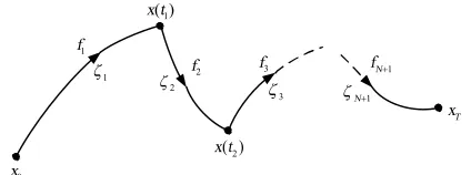
where N is the switching number; areattached together to steer the system to the target. In other words, N+1arcs are generated due to the given constant control inputs. It should be noticed that the number of arcs is one more than the number of switching. The final time tf in this case is chosen free.
Accordingly, a bang-bang control input can be defined as follows:
1 ( )
1, , 1
i
i i
u t u
i N
u+ u
= ì
= +
í =
-î K (2)
where, ui is the control input value in the itharc. Here,
the itharcis the trajectory segment x t( ) for
(
)
1,
i i
tÎ t- t ,
1, ,
i= K N whilst ti is the switching time. The
concatenation of these arcs is schematically illustrated in Figure 1.
1
z 1
f
0
x
T
x
2
z f2
1 N
z +
3 z
1 N
f+
3
f
1 ( )
x t
2 ( )
x t
The time duration of each arc is defined as follows:
1, 0,1, , 1
i ti ti i N
z = - - = K + (3)
In other words, ziis the elapsed time to move through the ith arc. The vector N1
R
zrÎ + is defined as follows:
[
1, , ,2 N1]
zr= z z Kz + (4)
In fact, time optimal bang-bang control problem of system (1) in the MIPSO-SQP algorithm is considered as follows:
1 1
minimize ,
subject to ( ) N
MIPSO SQP f i
i
f T
P t
x t x
z +
-=
= =
=
å
(5)where, the switching number (N) and the control input in each arc (ui) is assumed unknown. Problem in (5)
can be viewed as a problem of solving an optimization problem with equality constraint. To solve this problem, first the equality constraint x t( )f =xT is added to the objective function in (5) as a penalty function to reduce the problem to an unconstrained one. Then MIPSO-SQP algorithm is used to minimize the new altered objective function. Consequently, time optimal bang-bang control problem for system (1) is proposed as follows:
(
)
1 2
1 1
minimize ( )
j
N n
MIPSO SQP i j j f T
i j
P - +z a x t x
= =
ì
=í +
-î
å å
(6)where, ziis the time duration of the ith arc,
j
a is the weighting factor, N is the switching number and n is the system order. x tj( )f and xTjare the real and the desired final value of the jth state variable, respectively. It can be
seen that any deviation from the equality constraint will penalize the objective function. Now, the problem is to find the switching number (N), the optimal control input value in each arc and the time duration of each arc (
, 1,2, , 1
i i N
z = K + ) such that the new objective function
in (6) is minimized. This is already performed using PIPSO-SQP algorithm. However, in this paper the problem is solved using MIPSO-SQP in a more effective and systematic procedure.
3. IPSO-SQP ALGORITHM TO SOLVE
NONLINEAR OPTIMAL CONTROL PROBLEMS
3.1. IPSO Algorithm Particle swarm optimization (PSO) is inspired from movement and menuevring of birds. This algorithm was first improved by Eberhart and Kenedy in 1995 [8]. This algorithm uses the concept of social mutual effect in order to solve optimization problems. In this algorithm so called particles move in the search space to reach to a better
solution. Each particle is considered as a point in an N-dimensional space. The place is updated according to some past experiences of the particle, incorporating some other birds.
Particle moves according to its best value (called the personal best, pbest) in the search space. The other best value which is found by the crowed is called the global (or local) best (gbest or lbest, respectively). Indeed, the PSO is involved with the acceleration of each particle from the pbest towards the gbest (lbest) using an inertia weight.
At the starting, the number of population is randomly created in the given search space. Each particle uses its own velocity vector which is updated at any iteration according to:
(
)
(
)
1
1 1 2 2
k k k k k k
i i i i i
v+ =wv +c r pbest -x +c r gbest -x
(7)
where, k i
x is position of ith particle in kth iteration,
using w as the inertia weight. Scalar c1 and c2 are the acceleration coefficients, ri is a random uniformly distributed number in the range
[ ]
0,1 . Thereafter position of each particle is updated as follows:1 1
k k k
i i i
x+ =x +v+ (8)
These update laws in (7) and (8) are repeated until a stopping criterion in the algorithm is met. In order to get the algorithm always alive, a weighting factor is proposed to prevent the algorithm to stuck in a local minima. Preventing the PSO algorithm to stick in a local minimum, the weighting factor is proposed in Eq. (9) [6] is updated as follows:
(
1 exp( 1 ( )))
k
i k
i
w
F pbest
a
=
+ - (9)
Furthermore, another coefficient is also proposed to adjust the speed of convergence as a=1 (F gbest). These Improved PSO (IPSO) algorithms are finally called IPSO.
3.2. SQP Algorithm
SQP as a gradient based technique is an iterative analytical nonlinear programming method. This technique begins from an initial guess to find a solution according to the gradient information. This optimization method is found faster than other population based search algorithms.
Consider an optimization problem in the following inequality restricted form:
minimize ( )
subjected to i( ) 0, 1, 2, ,
J x
x i l
y
ì
í £ =
î K (10)
technique. Among several technique, the SQP technique needs to establish a Lagrangian function L x( , )l in terms of the Lagrangian multiplierli. This is constructed considering the cost function together with the constraint according to the following form:
1 ( , ) ( ) m i i( )
i
L xl J x ly x
=
= +
å
(11)The usual SQP consists of three main parts [6]:
1- Construct the Hessian of the Lagrangian function according to:
1
T T
k k k k
k k T T
k k k k k
q q H H
H H
q s s H s
+ = +
-0
H =I
1
k k k
s =X+ -X
( ) ( )
( ) ( )
1 1
1
1
n
k k i i k
i n
k i i k
i
q f x g x
f x g x
l
l
+ +
=
=
= Ñ + Ñ
æ ö
- Ñç + Ñ ÷
è ø
å
å
(12)
This is in the literature called as the first derivative try.
2- Solve the following quadratic programming sub-problem:
1
min ( )
2
T T
k k k k k
d H d + Ñf x d
( )T ( ) 0 1, , i xk dk i xk i me
y y
Ñ + = = K
( )T ( ) 0 , ,
i xk dk i xk i me m
y y
Ñ + ³ = K
(13)
3- A linear search is taken place to find a solution for the next iteration:
1
k k k
X+ =X +ad (14)
The algorithm is iteratively performed until a stopping criterion (maximum iteration or a convergence criterion) is met.
It is worth noticing that parameter of the step length
k
a , is determined via a (linear) search procedure. More detail about SQP algorithm can be found in [9-12].
3. 3. IPSO-SQP Algorithm [7]
In the following, a
quick review of the IPSO-SQP algorithm as a combination of two techniques of IPSO and SQP is addressed. It is an aim to get benefits of both algorithms in a practical application. In this method, first a group of particles is randomly chosen. The IPSO is done to find a global best position. Then, the routine is switched to SQP algorithm to search around the found global best for possible alternative solutions. The combination is as follows:Step 1: Randomly initialize the position and velocities of particles.
Step 2: Assess the fitness amount (Performance index) of each particles.
Step 3: If the previusly defined maximum iteration is reached, go to step 7, else continue.
Step 4: Store the current achieved best global. If the difference between the current best global performance and the previous one is fewer than a predefined amount, go to step 7 else continue.
Step 5: Update velocity and position of all particles according to Eqs. (7) and (8).
Step 6: Update the inertia weight of each particle according to Eq. (9) and go to step 2.
Step 7: Switch to the SQP algorithm to search around the global best, which is found by IPSO. In this case, the best achived solution by IPSO is considered as an initial guess for the SQP algorithm.
4. PIPSO-SQP AND MIPSO-SQP ALGORITHMS
In this section, PIPSO-SQP and MIPSO-SQP algorithms are presented. These two algorithms use the IPSO-SQP algorithm as a core routine. However, the change is in the procedure that the IPSO-SQP is used to find the optimal control input and final minimum time. In the following, first the PIPSO-SQP algorithm is briefly introduced then MIPSO-SQP algorithm is proposed for solving time optimal bang-bang control problems. More detail about PIPSO-SQP can be found in [13-15].
4. 1. PIPSO-SQP Algorithm It is shown that the PIPSO-SQP algorithm is able to solve time optimal bang-bang control problems. The particles are the arc times and the sum of these arc times form the cost function. The equality constraint is added to the cost function as a penalty function and the aim is to minimize the augmented cost function in (6). The procedure of the IPSO-SQP algorithm for solving the time optimal bang-bang control is described in the following:
Step 1: Guess the number of switching N.
Step 2: Set the initial value of the control input
max
(0)
u =u .
Step 3: Find a possible solution with N times switching using the IPSO-SQP method and seti=1.
Step 4: Find a time optimal solution for N i+ and
N i- switching using the IPSO-SQP method.
Step 5: In the case of no improvement on tf, keep the obtained solution in step 3 as a possible optimal solution and go to step 6. Otherwise, set i= +i 1and go to step 4. Step 6: if u(0)= -umax assign a label S2to the solution
the label of the solution will be assigned asS1. Set
max
(0)
u = -u and go to step 3.
Step 7: Among the sets of the solution S1 and S2, select the answer with the minimum time tf and regard it as the desired solution and stop.
Flowchart of the method is depicted as follows:
max (0) u =u
1
i=
N i- N i+
f t
max (0) u = -u
max (0) u = -u
max (0) u =u
1 i i= +
max (0) u = -u
Infact, to gain this procedure, value of the switching number is primarily guessed. Thus, for an initial control input (u(0)= +umax) the algorithm is executed to find an optimal arc times. For a specific switching number N, the final time is improved. Then, the algorithm searches for best solution forN+1 and N-1 switching.
Similarly, the solution is assessed for a possible improvement. If so, the algorithm is again performed for
2
N+ and N-2 switching. The procedure continues
until improvement in final time is not of the case. In this case, the current result is stored as the best. Again the algorithm is run for some other initial control input (u(0)= -umax) for the same initial guess of the switching number i.e. N. Accordingly, the procedure is repeated for the new guess. Consequently, the so called best achieved results for each initial control input are
compared to find the less final time. Ultimately, the achieved time is considered as a solution of time optimal bang-bang control problem.
4. 2. MIPSO-SQP Algorithm
The IPSO-SQP algorithm is used in a specified procedure for solving time optimal bang-bang control problem (PIPSO-SQP algorithm). However, the proposed MIPSO-SQP algorithm finds the optimal bang-bang control input in another way, which is more general and effective than the PIPSO-SQP algorithm. In MIPSO-SQP algorithm, the switching number, N and the initial control input
1
(0)
u =u are primarily guessed. The value of the control input for the rest of arcs is determined according to (2). In the algorithm, the arc times are considered as particles. Namely the time duration of each arc are updated in the optimization process until for a number of arcs with specified time duration the system reach to the target in minimum time. Accordingly, the dimension of each particle depends on the switching numbers. In fact if the switching number is assumed N, then N+1 arc is generated and the dimension of each particle will be
N+1 (d=N+1). For each dimension, which is the time
duration of an arc, an upper and a lower bound are determined. Since time is a nonnegative quantity, the lower bound can be assumed zero. However, it should be avoided to choose zero value for the lower bound. This is because it yields a numerical error in the running process of the program. Thus, the value of 10-6 is
considered for the lower bound in the IPSO-SQP algorithm. The procedure of MIPSO-SQP algorithm to solve the time optimal bang-bang control problem is summarized as follows:
Step 1: Initiate the switching number, N; and the initial value of the control input arbitrarily. Determine the maximum iteration and the switching criteria.
Step 2: Initialize the position and velocity of each particle.
Step 3: Execute the control system in (1) and evaluate the fitness function on (6) for each particle.
Step 4: If the maximum iteration criterion is met, go to step 8, otherwise; go to step 5.
Step 5: Evaluate and store the global and personal best. If the change between the current global best and its previous one is smaller than a pre-defined value, go to step 8, otherwise continue.
Step 6: Evaluate the inertia weight for each particle. Step 7: Update the particles velocity and position and go to step 3.
Step 8: The achieved global best using the IPSO algorithm is used as an initial guess for the SQP algorithm. Switch to use the SQP algorithm to search around the found global best.
Step 10: If there is no arc with zero length, add an arc to the begging and another arc to the end of the previous arcs and go to step 2.
Step 11: Consider the global best as the optimal solution and stop.
In fact, at the above procedure, step 2 to step 8 is iteratively repeated. If after running the algorithm, the obtained solution fails to satisfy the problem equality constraint, two arcs must be added to the previous arc. One to its beginning and the other to its end, then the algorithm goes back to step 2 and step 2 to step 8 is repeated for the new arcs. If the equality constraint is not again satisfied, two arcs are accordingly added. This procedure continues until the equality constraint is met. Then, zero arcs are tried to be found (arcs with zero length). If the solution doesn’t involve any zero arc, two arcs are added again to the previous arcs in the same manner to make sure that better solution (smaller tf) is not yet achieved for more arcs. In parallel, two arcs must be added as well. This procedure continues until the arc with zero length is achieved. This means there is no better solution for more number of arcs. Based on the described procedure for the MIPSO-SQP algorithm, for an initial guess of switching number; the MIPSO-SQP algorithm finds the global optimal solution in less iterations. This is because an additional calculations like running the control system and evaluating the fitness function for both initial control input and for both number of switching (N+i and N-i) is swapped the action of just adding arcs to the previous one.
Flochart of the MIPSO-SQP algorithm is depicted as follows:
By comparing the flocharts for PIPSO-SQP and MIPSO-SQP algorithm, it can be seen that MIPSO-SQP algorithm routinly finds the solution in a more systematic way. In the following advantages of MIPSO-SQP algorithm is numerically verified in a time optimal bang-bang control of some nonlinear systems.
5. USE OF MIPSO-SQP ALGORITHM IN TIME OPTIMAL BANG-BANG CONTROL OF SOME NONLINAR SYSTEM
In this section, to verify the performance of the proposed MIPSO-SQP algorithm, it is gained on a time optimal bang-bang control of Van Der Pol equations, Rayleigh system and an F8 aircraft model. The results are compared with those obtained using gradient-based method and PIPSO-SQP algorithm.
5. 1. Van Der Pol Equation
The Van Der Pol dynamic is described by:
(
)
1 2
2
2 1 1 1 2
x x
x x x x u
=
= - - - +
&
& (15)
where, the control input is bang-bang and can be defined as
{
u u u1, , ,2 3K} {
= -1, 1,1,K}
or{
u u u1, , ,2 3K} {
= -1,1, 1,- K}
. The initial and final point ofnot singular solution are set to x0=
[ ]
1,1 and xT =[ ]
0, 0respectively [1].
In the following, three different methods are applied to solve this time optimal bang-bang control problem.
5.1.1. Time Optimal Switching Method (TOS) The problem mentioned above is solve in [1] through using a gardeint-based method called TOS. This method is highly dependent to the initial guess of the solution and needs to be start from a feasible point. Thus, it applies another method to provide a feasible starting point. In [1], the STC method is primarily used to give in hand the starting point. The STC method found the arc and final times as z=
[
3.92540, 0.43500, 3.28560]
and7.64600 f
t = respectively [1]. The distance from the origin was also0.00037. Using the outcome of the STC
technique as an initial guess of the TOS achieves
[
0.7230, 2.37220]
z = and tf =3.09520 for the arc times and the final time, respectively [1]. These results provide a fewer distance to the final states from the origin of order10-4. In fact, the length of third arc was
5.1.2. PIPSO-SQP Algorithm Further results of using PIPSO-SQP algorithm is presented in other work. First, the algorithm is initialized by setting parameters c1 and c2in the IPSO algorithm to: c1=c2=2 [16]. Particles are the arc times. Population size is also set
60
s= . Each dimension of particle is supposed bounded ( 10 ,56
i
z é - ù
Î ë û seconds). Meanwhile, particles are randomly distributed around the centre of the search space by uniform distribution. For initial guess ofN =4, in the first iteration, PIPSO-SQP algorithm searches the solution for
{
u(0) 1, = N=4, N=5, N=3}
. It must be mentioned that the algorithm is executed 20 times for each switching number. In step 5, the value of counter i is increased and the algorithm returns to the step 4 to find the best solution for{
u(0) 1, = N=2, N=6}
. However, in step 5, no improvement is detected for the final time. Thus, the best solution achieved for u(0) 1=is stored. The mentioned procedure is schematically as follows:
2 6
(0) 1, 4 4
5
N=3
N N
u N N
N
ì ì =
í
ï =
î ïï
= = í =
ï = ï ïî
The results at this stage are presented at Table 1. At this table, "N" represents the number of switching. Meanwhile, (B), (M) and (W) define the best, Mean and worst results for final time in 20 tries of the algorithm, respectively.
Then, the algorithm moves to step 6 and similarly searches the solution for {u(0)= -1, N=4, N=5, N=3}. Due to improvement in the final time, in step 5 i is incremented once and the algorithm goes back to step 4 to search for solutions
{
u(0)= -1, N=2, N=6}
. Again, in step 5 the improvement in the final time is observed.Thus, i is execute the best solution for
{u(0)= -1, N=1, N=7}. Better final time is achieved for
{
u(0)= -1, N=1}
, thus i is increased again and the algorithm searches the solution for{
u(0)= -1, N=8}
. This time, the final time is seen not improved. Therefore, the best result, which is achieved for{
u(0)= -1, N=1}
is stored. The mentioned procedure is schematically shown as follows:{ 8
7 6
(0) 1, 4
4 5
N=1 N=2 N=3
N N N
u N
N N
ì ì ìï =
ï ï í
= í ï
ï î
ï ïï î = = - = í
ï ï = ï ï = î
The results in this case are presented in Table 2.
TABLE 1. Results of using PIPSO-SQP algorithm in Van Der Pol equation (u(0) 1= )
(0) 1
u =
N B M W
2 3.1178 3.3216 4.9957
3 3.0973 3.2675 4.8553
4 3.1501 3.8943 5.4872
5 3.3596 4.0105 5.5178
6 5.1427 5.2769 5.6553
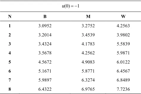
TABLE 2. Result of using PIPSO-SQP algorithm in Van Der Pol dynamics considering (u(0)= -1)
(0) 1
u =
-N B M W
1 3.0952 3.2752 4.2563
2 3.2014 3.4539 3.9802
3 3.4324 4.1783 5.5839
4 3.5678 4.2562 5.9871
5 4.5672 4.9083 6.0122
6 5.1671 5.8771 6.4567
7 5.9897 6.3274 6.8489
8 6.4322 6.9765 7.7236
Finally, in the algorithm goes to step 7 and compares the solution for both u(0) 1= and u(0)= -1 (from the results presented in Tables 1 and 2). The best achieved result using the PIPSO SQP method is for one time of switching (N=1) and the control input as u= -{ }1,1 , the arc times are z =
{
0.7230, 2.3717}
and the final time is3.0952
f
t = .
As it is obvious from Tables 1 and 2, for the initial guess of N=4 the algorithm first searches for the possible solution for u(0) 1= . The best results in this case is achieved for
{
u(0) 1,= N=3}
. Then, the algorithm goes to step 6 to search the possible best solution for u(0)= -1. In this case, the algorithm tries different value of the switching number because of meeting improvement in the final time. The best results in this case is achieved for {u(0)= -1,N=1}. At last, by comparing the both best achieved results of{u(0) 1,= N=3} and
{
u(0)= -1,N=1}
, the algorithms gives the solution of time optimal problem as :{ }
{ }
1, 1,1
0.7230, 2.3717 3.0952
f
N u
t z
= = -ì
ï = í ï = î
different switching numbers while the initial control input is assumedu(0)= -1 and similarly foru(0) 1= . This is a time consuming task, which needs several calculations and function evaluations. However, in the following the MIPSO-SQP will be shown able to find the global optimal solution for initial guess of N=4
just by one time running of the algorithm.
5.1.3. MIPSO-SQP Algorithm In this section, the proposed MIPSO-SQP algorithm is used for time optimal bang-bang control of Van Der Pol equation. Parameters c1 and c2 is set to: c1=c2=2 [16]. The
population size and the upper and lower bounds are also set to 60 (s=60) and 10 ,56
i
z é - ù
Î ë û respectively. Then, the particles are randomly initialized. The IPSO algorithm switches to the SQP algorithm when the change in the cost function value is lower than 0.0001 for ten successive iterations. For the initial guess of
{
u(0) 1,= N=4}
the algorithm is run 20 times. The results are presented in Table 3.According to the result in Table 3, for the initial guess of {u(0) 1,= N=4} the algorithm finds the best solution by making the length of the first and the fourth arc zero. This means the first and second arcs can be merged together as one arc with( ) 1
u t = (because the length of the first arc which is correspondent to u t( ) 1= is zero). Similarly, the third, fourth and the last arc can be again merged as one arc with u t( )= -1. This is because the length of the fourth arc which is correspondent to u t( )= -1is zero. This implies that the control input u t( ) 1= is kept unchanged from third arc to the last one.
Thus, the best result is yielded as follows:
{ }
{ }
1 1,1
0.7230, 2.3717 3.0952
f
N u
t
z
= ì ï = -ï í = ï ï = î
As previously stated, reaching the target is possible by one switching (N=1) and the control input of the form
{ }
( ) 1,1
u t = - .The optimal arc times and the final times are z =
[
0.7230, 2.3717]
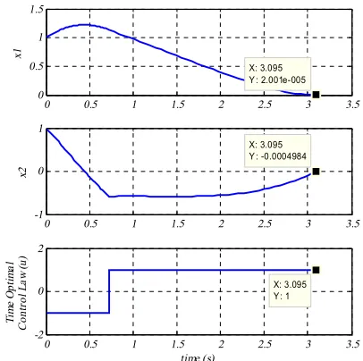
and tf =3.0952 respectively. The states trajectory of the best solution and the control input is depicted in Figure 2. The distance of the states from the final value is also shown in this figure.5.1.4. Comparison of the Methods As was mentioned before, for time optimal bang-bang control of Van Der Pol system, three different methods is applied. The first which was gradient-based method is very sensitive to the starting point. The initial guess of the solution in TOS algorithm must be feasible otherwise it fails to find the optimal solution. This algorithm needs
another algorithm to provide an appropriate starting point otherwise it can’t be efficient. From Table 3, can be seen that the algorithm finds a best solution by trying only one switching number i.e. N=4 which was initially assumed. It must also be mentioned that for this initial guess i.e.
{
u(0) 1,= N=4}
, MIPSO-SQP algorithm needs not to try other switching number. In contrast, PIPSO-SQP algorithm in a similar condition (namely {u(0) 1,= N=4}) tries N=2, N=3, N=4,5
N= and N=6 independently to find possible improvement in final time. Furthermore, PIPSO-SQP
algorithm needs to be executed for
{u(0)= -1,N=1, 2,3, 4,5, 6, 7,8} to compare the final
achievement best solutions. Indeed, for the initial guess of N=4 in PIPSO-SQP algorithm, the algorithm is tried 13 different cases of switching number (five different switching number for u(0) 1= and 8 different switching number for u(0)= -1). Contrarily MIPSO-SQP algorithm is performed only for one switching number (that was initially guessed) namelyN=4. In conclusion, this significantly reduces the execution time and the size of calculations to make the algorithm convenient in real time applications.
Figure 2. x1 and x2 state trajectories and time optimal control input
TABLE 3. Results of using MIPSO-SQP algorithm in Van Der Pol equation (u(0) 1= )
(0) 1
u =
Optimal control input & arc time W
M B N
{ }
( ) 1, 1,1, 1,1
u t = -
-{
10 , 0.7230, 0.0773,10 , 2.29496 6}
z
-
-= 3.5981 3.1143 3.0952
4
0 0.5 1 1.5 2 2.5 3 3.5
0 0.5 1 1.5
X: 3.095 Y : 2.001e-005
x1
0 0.5 1 1.5 2 2.5 3 3.5
-1 0 1
X: 3.095 Y : -0.0004984
x2
0 0.5 1 1.5 2 2.5 3 3.5
-2 0 2
X: 3.095 Y: 1
Ti
m
e
O
pt
im
al
C
on
tr
ol
L
aw
(u)
However, to show the performance of the proposed MIPSO-SQP algortithm, it is run for different value of the initial switching number and for both u(0) 1= and
(0) 1
u = - . The results are presented in Tables 5 and 6. The parameters which are bold represent the added arcs. As it is seen from Tables 4 and 5, the proposed MIPSO-SQP algorithm is able to find the global optimal solution for all guess of switching number as follows:
{ } { } 1 1,1 0.7230, 2.3717 3.0952 f N u t z = ì ï = -ï í = ï ï = î
Now, the results of using MIPSO-SQP algorithm are investigated in detail. Consider the case forN=4 in Table 5 for example. One may see:
TABLE 4. Results of using MIPSO-SQP algorithm in Van Der Pol equation (u(0) 1= )
(0) 1
u =
Optimal control input& arc time W
M B N
{ }
( ) ,1, 1,
u t = -1 - 1
{
0.7230, 2.3722,10 ,106 6}
z= -
-85% 11.4165 3.095
1
{ }
( ) 1, 1,1
u t =
-{
10 , 0.7230, 2.37226}
z=
-100%
-3.095
2
{ }
( ) 1, 1,1, 1
u t = -
-{
10 , 0.7230, 2.3722,106 6}
z= -
-90% 8.7580 3.095
3
{ }
( ) 1, 1,1, 1,1
u t = -
-{10 , 0.7230,0.0773,10 , 2.29496 6 }
z - -= 45% 13.0828 3.095 4
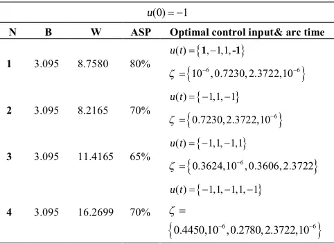
TABLE 5. Result of using MIPSO-SQP algorithm in Van Der Pol equation (u(0)= -1)
(0) 1
u =
-Optimal control input& arc time ASP
W B
N
{ }
( ) , 1,1,
u t = 1- -1
{
10 , 0.7230, 2.3722,106 6}
z= -
-80% 8.7580 3.095
1
{ }
( ) 1,1, 1
u t = -
-{
0.7230, 2.3722,106}
z=
-70% 8.2165 3.095
2
{ }
( ) 1,1, 1,1
u t = -
-{
0.3624,10 , 0.3606, 2.37226}
z=
-65% 11.4165 3.095
3
{ }
( ) 1,1, 1,1, 1
u t = - -
-{
0.4450,10 ,0.2780, 2.3722,106 6}
z - -= 70% 16.2699 3.095 4 { }
{
6 6}
4
1 , 1 , 1 , 1 , 1
0.4450,10 ,0.2780, 2.3722,10 3.0952
f
N u
t
z -
-ì = ï
= - -
-ï
ï ¯ ¯ ¯ ¯ ¯
í ï = ï ï = î
Since the best solution is achieved for one switching (N=1) and considering the control input u t( )={ }1, 1- , the length of the second and last arc is getting zero. In fact, the combination of the first three arcs acts as one arc where the control input is u t( )= -1 and the combination of the last two arcs acts as one arc where the control input is u t( ) 1= . It means that the system converges to the target by one switching and the control input of the form u t( )= -{ }1,1 . It must be mentioned that the best solution does not necessarily achieved by making the second and the last arc zero. Because the algorithm is heuristic, so each time for finding the global optimal solution, it assigns a value to each arc. To clarify the problem, the other best solution that is achieved for
4
N= is investigated as an example:
{ }
{
6 6 6}
4
1 , 1 , 1 , 1 , 1
10 ,10 ,0.7230, 2.6115,10 3.0952
f
N u
t
z - -
-ì = ï
= - -
-ï
ï ¯ ¯ ¯ ¯ ¯
í ï = ï ï = î
In this case, the length of the first, second and last arc is zero. It can be seen that, the third and fourth arc which is correspondent tou t( )= -1 and u t( ) 1= respectively are a nonzero amount and represent that the optimal solution is achieved for one switching and for
{ }
( ) 1,1
5.2. Rayleigh Problem The Rayleigh problem arises from such so-called tunnel diode oscillator, which is an electric circuit [5]. Consider the system as follows:
(
)
1 2
2 2 1 2 1.4 0.142 4
( ) 1 x x
x x x x u
u t
=
= - + - +
£
&
& (16)
State variable x1denotes a certain electric current, and the control input u the voltage of the generator in the circuit. The initial and final points together with the control signal are defined as:
[
]
0 5, 5
x = - - , xT=[ ]0,0 and { }
( ) 1,1
u t Î - respectively. The aim is to minimize the
following mixed cost function:
(
)
21 0
( ) (1 ) tf
f
J u t = +c t +
ò
x dt (17)The parameter “c” is set to c=1 16 [5].
The time optimal control that has been reported for this system is of bang-bang type, and this motivated us to apply the PIPSO-SQP and MIPSO-SQP algorithm to find the bang-bang constrained time optimal control for Rayleigh system. Meanwhile, for more comparison; the results obtained using the mathematical programming method is also presented.
5. 2. 1. Mathematical Programming Method The
results obtained using mathematical programming method is presented in [5]. First, the starting point is considered as u(0) 1= and z=
[
1.5, 2, 1, 0.5]
. The algorithm is run for this initial guess and the result is reported as:[
1.47614, 1.76069, 1.76069, 0]
z= and tf =3.773841
It can be seen that the time duration of the last arc is found zero that means two switching is enough for reaching the target.
It is mentioned in [5] that the mathematical programming method is highly dependent to the starting point. The initial guess must be chosen very close to the optimal results which need the designer to be very familiar with the problem. Another disadvantage of this method is the need to many derivative information of the cost function which may be troublesome in complex system or when the designer is not very familiar with the problem to find a good initial guess.
5.2.2. PIPSO-SQP Algorithm PIPSO-SQP algorithm is applied for time optimal bang-bang control of Rayleigh system. Initialization part is the same as the Van Der Pol time optimal problem. An initial guess of the switching number is assumed N=4. The algorithm
searches for optimum solution for
{u(0)= -1, N=4, N=5, N=3}. The results are presented in Table 7.
3 (0) 1, 4
5
N=4
N
u N
N
= ì ï
= - = í
ï = î
In step 5, the obtained results (Table 6) are evaluated and since there is no improvement in result, the algorithm returns to step 6 to search for the solution of
{
u(0) 1, = N=4, N=5, N=3}. The same procedure continues to find the best solution. Because of the improvement in the final time, in step 5, i is increased and the algorithm goes back to step 4 to find the best solution for {u(0) 1, = N=2, N=6}. The final time isagain improved, so the value of i is increased in step 5 and the algorithm is performed to find the best solution for the new value of switching number namely
{u(0) 1, = N=1, N=7}. This time no improvement is detected for the new switching numbers.
1
3 7
6
(0) 1, 4 4
5
N=2
N
N N
N
u N N
N
ì ì ì =
ï = ï í =
í î
ï ï
ï î =
ïï
= = í =
ï = ï ï ï ïî
The results are presented Table 7.
TABLE 6.
Result of using PIPSO-SQP algorithm in Rayleigh
system in the first guess of u(0)= -1.
(0) 1
u =
-N B M W
3 4.6789 4.9706 5.4373
4 4.1873 4.5692 4.8677
5 5.2514 5.5436 6.1753
TABLE 7.
Result of using PIPSO-SQP algorithm in Rayleigh
system using second guess; u(0) 1=
(0) 1
u =
N B M W
1 - -
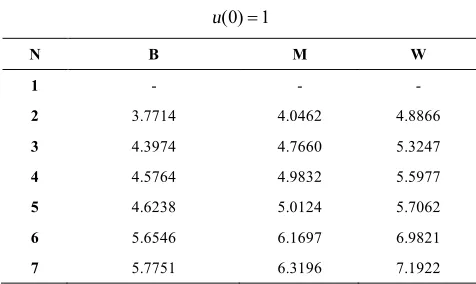
-2 3.7714 4.0462 4.8866
3 4.3974 4.7660 5.3247
4 4.5764 4.9832 5.5977
5 4.6238 5.0124 5.7062
6 5.6546 6.1697 6.9821
Comparing the achieved results for both u(0)= -1 and
(0) 1
u = verifies that best result is achieved as follows:
{ }
{ }
2 1, 1,1
1.4725,1.7649,0.5339 3.7714
f
N u
t
z
= ì ï = -ï í = ï ï = î
It is seen that for the initial guess of N=4 the algorithm is executed for three different switching number (
3, 4,5
N= ) while the initial control input is u(0)= -1 and is also run for seven different switching number (
1, 2,3, 4,5, 6,7
N= ) in case where the initial control input
is u(0) 1= . This is a time consuming task and involves additional calculations for finding the global optimal solution. However, MIPSO-SQP is able to find best solution for the same initial assumption just in one try of the algorithm.
5. 2. 3. MIPSO-SQP Algorithm The proposed MIPSO-SQP algorithm is used for time optimal bang-bang control of Rayleigh system. The arc times are the particles and are considered to be bounded ( 10 ,56
i
z é - ù Î ë û
seconds). The parameters c1 and c2 are set to 2 [16]. The
population size is set 60 (s=60). The IPSO algorithm switches to the SQP algorithm when the change in the cost function value is lower than 0.0001 for ten successive iterations. The algorithm is run for the initial guess of
{
u(0) 1,= N=4}
and the result is presented in Table 8. It can be seen from Table 8 that two switching is needed to steer the Rayleigh system to the target. The global optimal solution is as follows:{ }
{ }
2 1, 1,1
1.4725,1.7649,0.5339 3.7714
f
N u
t
z
= ì ï = -ï í = ï ï = î
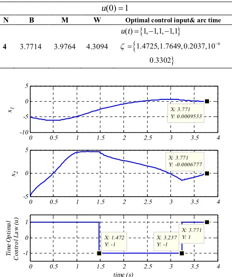
The state trajectories together with the time optimal bang-bang control input are depicted in Figure 3. The distance of the states from their final value is also shown in the figure. It can be seen from Figure 3 that using the MIPSO-SQP algorithm the states are steered from the initial point to the final point in the minimum time of 3.7714 seconds. As it is illustrated in the figure, the distance of thex1 andx2 state variables from their final value is 0.001425 and 0.0002906, respectively which is very close to zero.
5. 2. 4. Capability of the Applied Algorithms in a Rayleigh System Similar comparison will be made here when the Rayleigh system is under the control. The mathematical programming method which is very sensitive to the initial guess is used to find the time optimal control solution. The starting point must be
assumed very close to the final optimal solution to make the algorithm capable for finding the optimal solution. This drawback fails the algorithm to be used in cases where the designer is not very familiar to the problem. Moreover, the derivative information of the cost function causes the algorithm to be hardly useable for complex problems.
For the PIPSO-SQP and MIPSO-SQP algorithm, The switching number is initially considered as N=4, the PIPSO-SQP algorithm finds an optimal solution in many excessive tries. In fact, the algorithm is executed for three different switching numbers of N=3, 4,5when
(0) 1
u = . Similarly, the code is performed for seven different switching numbers of N=1, 2,3,4,5,6,7 for
(0) 1
u = - . At last by making comparison of the results obtained for both u(0) 1= and u(0)= -1the one with less achieved final time is considered as an optimal solution of the problem (i.e. u(0) 1,= N=2). However, MIPSO-SQP algorithm in the same condition i.e. initial guess of N=4, finds the global optimal solution only by making the length of some arcs zero whether the initial control input is assumed u(0) 1= or u(0)= -1. In deed, there is no need to try other value of switching number to find an optimal solution.
TABLE 8. Result of using MIPSO-SQP algorithm in Rayleigh system ( (0) 1u = )
(0) 1
u =
N B M W Optimal control input& arc time
4 3.7714 3.9764 4.3094
{ }
( ) 1, 1,1, 1,1
u t = -
-{
}
6 1.4725,1.7649, 0.2037,10
0.3302
z=
-Figure 3. The state trajectories x1 and x2, and optimal control input
0 0.5 1 1.5 2 2.5 3 3.5 4
-10 -5 0 5
X: 3.771 Y: 0.0009533
x1
0 0.5 1 1.5 2 2.5 3 3.5 4
-5 0 5
X: 3.771 Y: -0.0006777
x2
0 0.5 1 1.5 2 2.5 3 3.5 4
-1 0 1
X: 3.771 Y: 1
Ti
m
e
O
pt
im
al
C
on
tr
ol
L
aw
(u)
time (s)
X: 3.237 Y: -1 X: 1.472
This ultimately reduces the computation time and additional calculation. In the following, to show the performance of the proposed algorithm it is run for different value of switching number and for both initial value of the control input. The best and worst results are presented in Tables 9 and 10. The number of times in percentage that the algorithm is able to find the best solution during 20 times running of the algorithm is explained through the parameter ASP. Notice that the values which are bold represent the added arcs.
TABLE 9. Results of using MIPSO-SQP algorithm in Rayleigh system considering (0) 1u =
(0) 1
u =
N B M W Optimal control input& arc time
1 3. 7714 3.9368 4.2670 u t( )={-1,1, 1,- 1}
{
10 ,1.4725,1.7649,0.53396}
z=
-2 3. 7714 3.8932 4.1156
{ }
( ) -1,1, 1,1,-1 u t =
-{
10 ,1.4725,1.7649,0.5339,106 6}
z
-
-=
3 3. 7714 4.1129 4.5721 u t( )={1, 1,1, 1- -}
{1.4725,1.7649, 0.5339,106}
z=
-4 3.7714 4.1761 4.613
{ }
( ) 1, 1,1, 1,1
u t = -
-{1.4725,1.7649, 0.2037,10 , 0.33026 }
z
-=
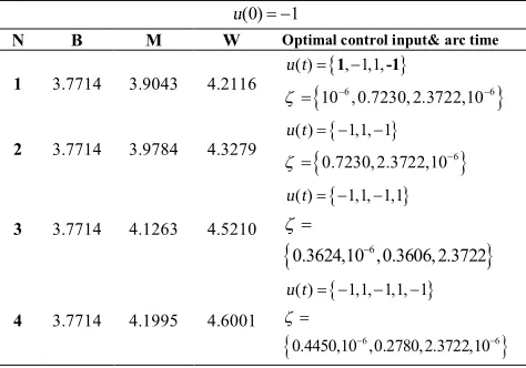
TABLE 10. Results of using MIPSO-SQP algorithm in Rayleigh system (u(0)= -1)
(0) 1
u =
-Optimal control input& arc time W
M B
N
{ }
( ) , 1,1,
u t = 1- -1
{
10 , 0.7230, 2.3722,106 6}
z= -
-4.2116 3.9043
3.7714
1
{ }
( ) 1,1, 1
u t = -
-{
0.7230, 2.3722,106}
z=
-4.3279 3.9784
3.7714
2
{ }
( ) 1,1, 1,1
u t = -
-{
0.3624,10 ,0.3606, 2.37226}
z
-=
4.5210 4.1263
3.7714
3
{ }
( ) 1,1, 1,1, 1
u t = - -
-{
0.4450,10 ,0.2780,2.3722,106 6}
z
-
-=
4.6001 4.1995
3.7714
4
6. CONCLUSION
In this paper, MIPSO-SQP algorithm is proposed to solve a time optimal bang-bang control problem. Various steps of the algorithm for solving time optimal bang-bang control problem is described. The proposed
MIPSO-SQP algorithm is found more effective in comparison with the time optimal switching control method (TOS), mathematical programming method and PIPSO-SQP algorithm. This algorithm is able to find global solution in spite of different initial guess for switching number and control input. MIPSO-SQP finds global optimal solution more systematically and in less number of times of algorithm try. In fact, using the proposed MIPSO-SQP algorithm, global optimal solution is achieved for wider range of initial guess of the control input together with number of the switching. Performance of the proposed MIPSO-SQP algorithm is verified through applying the algorithm in time optimal bang-bang control problems of Van Der Pol equation, Rayleigh system and F8 aircraft model. Significance of the achievement is found when the result is compared with those obtained using the PIPSO-SQP algorithm.
7. REFERENCES
1. Kaya, C. Y. and Noakes, J. L., "Computational method for time-optimal switching control", Journal of Optimization Theory
and Applications, Vol. 117, No. 1, (2003), 69-92.
2. Penev, B. G. and Christov, N. D., "A fast time-optimal control synthesis algorithm for a class of linear systems", in American Control Conference, IEEE. (2005), 883-888.
3. Ebrahimi, A., Moosavian, S. A. A. and Mirshams, M., "Minimum-time optimal control of flexible spacecraft for rotational maneuvering", in Control Applications, IEEE International Conference on, IEEE. Vol. 2, (2004), 961-966. 4. Bayón, L., Grau, J., Ruiz, M. and Suárez, P., "Initial guess of the
solution of dynamic optimization of chemical processes",
Journal of Mathematical Chemistry, Vol. 48, No. 1, (2010),
28-37.
5. Kaya, C. Y., Lucas, S. K. and Simakov, S. T., "Computations for bang–bang constrained optimal control using a mathematical programming formulation", Optimal Control Applications and
Methods, Vol. 25, No. 6, (2004), 295-308.
6. Modares, H. and Naghibi Sistani, M.-B., "Solving nonlinear optimal control problems using a hybrid IPSO–SQP algorithm",
Engineering Applications of Artificial Intelligence, Vol. 24,
No. 3, (2011), 476-484.
7. Parsopoulos, K. E. and Vrahatis, M. N., "Recent approaches to global optimization problems through particle swarm optimization", Natural Computing, Vol. 1, No. 2-3, (2002), 235-306.
8. Kennedy, J., "Particle swarm optimization, in Encyclopedia of machine learning", Springer, (2010), 760-766.
9. Wang, X., Zhu, Z., Zuo, S. and Huang, Q., "An SQP-filter method for inequality constrained optimization and its global convergence", Applied Mathematics and Computation, Vol. 217, No. 24, (2011), 10224-10230.
10. Zhu, Z., Zhang, W. and Geng, Z., "A feasible SQP method for nonlinear programming", Applied Mathematics and
Computation, Vol. 215, No. 11, (2010), 3956-3969.
11. Alsumait, J., Sykulski, J. and Al-Othman, A., "A hybrid ga–ps–
12. Shen, C., Xue, W. and Chen, X., "Global convergence of a robust filter SQP algorithm", European Journal of Operational
Research, Vol. 206, No. 1, (2010), 34-45.
13. Taleshian T., Ranjbar A., and Ghaderi R., "Intelligent fractional order control of an autonomous underwater vehicle using IPSO-SQP algorithm", in 5th IFAC Symposium on Fractional Differentiation and Its Applications (FDA12). China. (2012) 14. Taleshian T., Ranjbar A., and Ghaderi R., Design of an optimal
tracking controller for an autonomous underwater vehicle using ipso-sqp algorithm, in Intelligent and Knowledge Technology Conference (IKT2012). (2012)
15. Taleshian T., Ranjbar A., and Ghaderi R., Optimal control of an autonomous underwater vehicle using ipso_sqp algorithm, in International Conference on Control, Instrumentation and Automation, (ICCIA2012), IEEE Index, (2012)
16. Shi, Y. and Eberhart, R., "A modified particle swarm optimizer", in Evolutionary Computation Proceedings, IEEE World Congress on Computational Intelligence. (1998), 69-73. 17. Banks, S. and Mhana, K., "Optimal control and stabilization for
nonlinear systems", IMA Journal of Mathematical Control and
Information, Vol. 9, No. 2, (1992), 179-196.
18. Kaya, C. Y. and Noakes, J. L., "Computations and time‐optimal controls", Optimal Control Applications and Methods, Vol. 17, No. 3, (1996), 171-185.
APPENDIX A
In this section the MIPSO-SQP algorithm is implemented on F8 aircraft model for more comparison. The achieved results are also compared with those obtained using some other methods. The following F8 aircraft model has widely been used in several control studies [1, 17, 18]:
2 2
1 1 3 1 3 1 2
2 3 2 2
1 3 1 1 1
3
2 3
2 3
3 1 3 1 1
2 2 3
1 1
0.877 0.088 0.47 0.019
3.846 0.215 0.28 0.47
0.63
4.208 0.396 0.47 3.56 20.967
6.265 46 61.4
x x x x x x x
x x x u x u x u u
x x
x x x x x u
x u x u u
= - + - +
-- + - + +
+ =
= - - - -
-+ + +
&
& &
(18)
where, x1 is the angle of attack in radians, x2and x3are the pitch angle and the rate in rad srespectively. The control input uis tail deflection angle. The initial and
final value of the states, and the control input are as follows:
(
)
(
)
{
}
0 180 26.7,0, 0 , 0, 0,0 , ( ) 3 ,3
T T
T
x = p x = u t Î - o o
The goal is to minimize the approach time that system is to steer from an initial condition to a target.
Mathematical Programming Method In [6], time
optimal bang-bang control of the F8 aircraft model is investigated using mathematical programming method. It was mentioned before that this algorithm is sensitive to the initial guess. Thus, the algorithm is run for different initial point and the best result is achieved for the initial guess of u(0) 3 ,= o z =
{
1, 0.3,1.5,1,1}
asfollows:
{
}
(0) 3 , 1.1327, 0.3475,1.6089,0.6924 , f 3.7815
u = o z = t =
It can be seen that the initial point is very close to the optimal solution. Therefore, it makes it hard to deal with this algorithm.
PIPSO-SQP Algorithm Primarily, the algorithm is initialized. Parameters c1 and c2 are set to 2.
Population size is set to 60 (s=60). The algorithm is similarly performed 20 times for initial guess of N=4
andu(0) 3= o, then the optimization procedure is
followed by trying the switching numberN=3and
5
N= foru(0) 3= o. A best result is achieved as
{
u(0) 3 ,= o N=3}
is also stored, i is increased and the algorithm returns back to step 4 to search for possible improved solution of{
u(0) 3 , = o N=2, N=6}
. Better finaltime is not achieved for the new value of switching number. Thus, the algorithm moves to step 6 to run for the same initial switching number namely N=4 but
(0) 3
u = - o.
2 3
6
(0) 3 , 4 4
5
N N
N
u N N
N
ì ì =
= í
ï =
î ïï
= = í =
ï = ï ïî
o
Similarly, the optimization process is followed by trying the switching number N=3 and alternativelyN=5.
3
(0) 3 , 4 4
5
N
u N N
N = ì ï = - = í =
ï = î o
Finally, by comparing the achieved results of applying two control inputs best result is achieved as follows:
{
}
{
}
3
( ) 3 , 3 ,3 , 3
1.1348,0.3464,1.6083, 0.6905 3.78
f
N u t
t z
= ì ï
= -
-ï í
= ï ï = î
TABLE A. 1.
Results of using PIPSO-SQP algorithm in F8
aircraft system, concerning u(0) 3= o.
(0) 1
u =
N B M W
2 - -
-3 3.78 3.9212 4.2396
4 4.3290 4.6368 5.1097
5 4.9548 5.3215 5.8675
6 5.7359 6.0573 6.5178
TABLE A. 2.
Results of using PIPSO-SQP algorithm in F8
aircraft system, choosing (0)u = -3o
(0) 3
u = - o
N B M W
3 4.4236 4.6712 5.2342
4 3.9943 4.3451 4.5373
5 4.9548 5.3215 5.8675
However, best result is achieved causing extra computation and function evaluations. Indeed, these are time-consuming tasks to run the algorithm for both initial control input and for different manoeuvring switching numbers. Specifically in case where the initial switching number is far from the correct value of the switching number, the algorithm needs to be executed several times for different switching numbers to find better results. However, in the following, the MIPSO-SQP algorithm is used to solve time optimal bang-bang control problem of an F8 air craft model to show capability of MIPSO-SQP to find best result for N=4
in just one try.
MIPSO-SQP Algorithm MIPSO-SQP algorithm is
applied in time optimal bang-bang control of an F8 aircraft model. Primarily, the algorithm is initialized i.e.
1 1 2
c =c = and s=60. The particles are the arc times and each dimension is bounded (z é10-6 5ù
Î ë ûseconds).
These initial particles are randomly distributed. The IPSO algorithm switches to the SQP algorithm when the change in the cost function value is lower than a predefined threshold e.g. 0.0001 for ten successive iterations. Accordingly, the best, the mean and the worst results are presented in Table A. 3. The best result is deduced as follows:
{
}
{ }
3
( ) 3 , 3 ,3 , 3
1.1348,0.3464,1.6083, 0.6905 3.78
f
N u t
t
z
= ì
ï = -
-ï í
= ï ï = î
o o o o
(19)
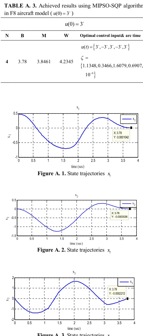
In fact, by three times switching of the control input and
consideringu(0) 3= ostates are steered from an initial
point to the target in minimum time (tf =3.78
seconds). State trajectories are illustrated in the following figures (Figures 5 to 7).
Final values of state variables are also stated in figures. It can be seen that the error of states from their final value is very close to zero.
TABLE A. 3. Achieved results using MIPSO-SQP algorithm in F8 aircraft model (u(0) 3= o)
(0) 3
u = o
Optimal control input& arc time W
M B N
{
}
( ) 3 , 3 ,3 , 3 ,3 u t = o-o o-o o
{
}
61.1348, 0.3466,1.6079, 0.6907, 10
z
-=
4.2345 3.8461
3.78
4
Figure A. 1. State trajectories x1
Figure A. 2. State trajectories x2
Figure A. 3. State trajectories x3
0 0.5 1 1.5 2 2.5 3 3.5 4
-1 -0.5 0 0.5
time (sec)
x1
x1
X: 3.78 Y: 0.0001042
x1
0 0.5 1 1.5 2 2.5 3 3.5 4
-1.5 -1 -0.5 0 0.5
x2
time (sec)
x2
X: 3.78 Y: -0.0003036
x2
0 0.5 1 1.5 2 2.5 3 3.5 4
-2 -1 0 1 2
x3
time (sec)
x3
X: 3.78 Y: -0.0002212
Efficiency of the Applied Algorithm in F8 Problem It is also shown in this case that the MIPSO-SQP algorithm is more effective to find time optimal bang-bang control input. As it was mentioned, the mathematical programming needs to be start from a point that is very close to the optimal solution, and needs many derivative information of the cost function for solving the time optimal bang-bang control problem. In addition, it can be seen from Table A. 3, for the initial guess of u(0) 3 ,= o N=4 the MIPSO-SQP algorithm is able to find the best solution by making the length of the last arc zero. On the other hand, it is found not sensitive to variation in the initial guess of the switching number or control input. However, for the same initial guess of the switching number namely
4
N= , PIPSO-SQP algorithm needs to try different decreasing and increasing value of switching number with respect to the initial guess (N=4) for both
(0) 3
u = o and u(0)= -3o. This finally yields PIPSO-SQP
algorithm to find a best solution in more iterations which makes the code more time consuming.
Using Modified IPSO-SQP Algorithm to Solve Nonlinear Time Optimal Bang-bang
Control Problem
T. Taleshian, A. Ranjbar, R. Ghaderi
Department of Cont