A b s t r a c t. The use of simplex algorithm for determination of soil aggregation extreme changes has been presented. It enables to find the range of changes of the soil aggregates stability index for one-directional aggregation changes and assigned criterion of the soil aggregation stability evaluation. The basic data for calculation of the ranges of changes are distributions of soil aggregate fre-quencies before and after the occurrence of the destruction factor. The problems of existence of feasible solutions and their unique-ness have been also discussed. It has been found that simplex algo-rithm is suitable for calculation of extreme values of aggregates stability index (ASI).
K e y w o r d s: simplex algorithm, soil aggregates, stability index
INTRODUCTION
Soil aggregates are classified according to their size. However, it is not only the temporary state of aggregation that decides about soil quality but also its variability. There-fore, the dynamics of changes of aggregation or the stability of aggregation is analyzed. From this point of view, soil ag-gregates can be characterized, either as being resistant or vulnerable (sensible) to the action of external factors. The pairs of these qualifications are dual to each other [1, 7].
The change in soil aggregates size is an inevitable con-sequence of natural processes and a specific tendency of soil aggregates change, i.e., decomposition or sticking together can be evaluated positively or negatively. External factors can affect soil aggregates randomly – independently from human intentions, or purposely – in agreement with our ex-pectations. In both cases, they can be short time actions (accidental events, agrotechnical treatments) or long time actions including the processes lasting several years [4, 11].
Niewczas and Witkowska-Walczak [10] proposed the soil aggregates stability index (ASI) for evaluation of
ag-gregation changes in a tested soil sample. It has been defined as a value of a function, which arguments are all the frequen-cies of the transition table. The coefficients of this function are respectively chosen weights assigned to each element of the transition table. The index, determined this way, is a me-asure of changes of aggregation within the whole soil sam-ple which took place during the input® output cycle and it emphasizes the importance of these changes through the given weights. In paper [10], the linear function was used and the weights were numbers with 2 as bases and integer exponents, which were adequated to the number of aggrega-te classes, of which the decrease of a given aggregaaggrega-te fra-ction occurred as a result of the afra-ction of a destructive factor. The definition of ASI enables to calculate its value for each aggregate class separately and the sum of these individual values is a value of the index of the whole soil sample. The-refore, the additivity of the measure of stability, determined this way, is preserved.
To find the extreme values of ASI the optimization me-thods can be used and especially the operations research [8, 9]. This group of methods contains, between others, the linear programming. It is a method usually used for optimi-zation of economical enterprises, however its mathematical foundations open the way to broad spectrum of possible applications.
The aim of this paper was to use the simplex algorithm for determination of soil aggregation extreme changes.
The method presented in this paper enables to obtain from available data some additional information about ag-gregation changes, which cannot be possessed with help of other known methods. None similar approach to the pro-blem of the analysis of changes of the soil aggregate stability has been found in the specialistic literature.
Use of simplex algorithm for determination of soil aggregation extreme changes
J. Niewczas* and B. Witkowska-Walczak
Institute of Agrophysics, Polish Academy of Sciences, Doœwiadczalna 4, P.O.Box 201, 20-290 Lublin 27, Poland
Received May 8, 2003; accepted May 29, 2003
© 2003 Institute of Agrophysics, Polish Academy of Sciences
*Corresponding author’s e-mail: [email protected]
A A
Agggrrroooppphhyhyysssiiicccsss w
w
THEORETICAL BASIS
Transition table
A detail analysis of aggregate changes can be done by writing the results of the performed experiment on the ag-gregates of a tested soil sample in form of a so-called tran-sition table from an input distribution (before the action of a destruction factor) to the output distribution (after the action of a destruction factor). The transition table is a form of the transition matrix, modified by the requirements of this study [5, 8]. It contains much more information about the changes of soil aggregates than the pair of their distributions at the input and the output. It shows how the particular classes of aggregates changed at input as the result of the investigated factor and what frequencies are included in the aggregate classes at the output.
The output soil material can be divided into classes and its changes at output can be investigated independently for each class. However, the analysis of the aggregates coming from successive classes at the input, does not give the insight into the distribution of the changes of a material quality in a given soil, unless it combines these classes through the knowledge of the frequencies of the aggregates appearance in a random sample, representing a given soil [6]. In nume-rous cases it does not matter how the aggregates convert from the input distribution to the output distribution and sometimes we are only interested in their output distribu-tion, i.e., the result of the action of a specific event, treatment or process. These are however, very simplified, utilitarian approaches. The knowledge of the behavior of all the aggre-gate classes (jointly), is very useful due to their hetero-geneity. The aggregates coming from different classes very often characterize with dissimilar inner structure and chemi-cal composition, and hence they do not react alike to the action of a destructive factor.
The necessary data for the stability analysis of the tested soil sample are the following relative frequencies:
pi. = [p1., p2., ..., pk.] – input distribution (before destruction
factor occurrence) of aggregate frequencies,
p.j= [p.1, p.2, ..., p.k] – output distribution (after destruction
factor occurrence) of aggregate frequencies
,
[pij] (i = 1, 2, ..., k; j = i, i+1, ..., k) – two-dimensional
distri-bution of aggregate frequencies; the numbers pijshow which weight portion of all mass of aggregates of the soil sample under the destruction factor remained in the same class (j=i) or which weight portion of those mass decomposed (j>i), turning from class i to one of the following classes, j. These data are obtained during the performed experiment.
Diagonal distribution, set of weights and soil aggregates stability index
In paper [10], the concept of a diagonal distribution diag= [d ,d ,... ,d0 1 k 1- ]as introduced. Its consecutive
fre-quencies d ,d ,... ,d0 1 k 1- are obtained by summing up the elements of the main diagonal of the transition table (their sum is denoted as d0) and the elements of succeeding diago-nals, which have the same distance from the main diagonal and gradually become more far away from it, thus the last frequency, dk 1- =p1k. According to the requirements of a frequency distribution, d0+ + +d1 ... dk 1-= 1. The form of a diagonal distribution gives information about the scale of changes of the aggregates of a studied soil sample as a result of an action of a destructive factor. The frequency d0, deter-minates, to the largest extent, the evaluation of the stability of a soil sample which has been under an action of a destru-ctive factor, whereas each succeeding frequency has smaller and smaller impact on it. Similarly, the magnitude of a num-ber in a positional notation is determined by its consecutive digits, starting from a left, most significant digit and ending at a right, the least significant digit.
To differentiate the importance of particular frequen-cies of a distribution diag, they were assigned to an appro-priately selected set of weights w=[w , w ,... , w0 1 k 1- ]. Using the above mentioned analogy of numbers notation in positional system, as a measure of stability of the aggregates composing the tested soil sample, an index ASI has been proposed, being a sum of products of the frequencies of the diagonal distribution and weights:
ASI=d w0 0+d w1 1+...dk 1-wk 1-. (1)
A system of binary weights was admitted: w0=2k 1-, w = 21 k 2- ,... , wk 1- =20. For k = 6 these weights take va-lues: 32, 16, 8, 4, 2, 1. Thus, the scale of ASI values is a range from 1 to 32.
Input and output frequencies distribution and a transition table
A transition of a sample elements of a material from the input frequency distribution to the output frequency distri-bution can be realized in different ways, through different ‘transition channels’ from one state (class) to another. The same pair of frequency distributions in the input and in the output can correspond to different transition tables. In Table 1, an appropriate example has been presented for four clas-ses of aggregates (fictitious data). Furthermore, it shows how different sums of frequency on a main diagonal (grey background) can be obtained for the same pair of input and output distributions. It leads to the conclusion that for given input and output distributions it is not possible to determine univocally their transition table except from specific cases (e.g., for unidirectional changes, when input and output distributions are identical or when one the distributions is reduced to one class). There can be many such tables. One of them is a table for a sample of a tested material, Ttest. The
point of view of an assumed criterion of evaluation of aggregate stability changes. Against the background of these tables (assigned further as Tminand Tmax, respecti-vely), a table Ttestwhich represents the changes of the
aggre-gation of an analyzed soil sample, which occurred between the input and the output can be evaluated. The data for
fin-ding the extreme transition tables are exclusively the frequ-ency distributions in the input (pi.) and in the output (p.j).
Under unidirectional changes, from all the possible transitions between two distributions, the frequencies p11 and pkkare always precisely determined – the first of them
through the input distribution and the second through the output distribution. These are the transitions: kl1® kl1and
klk® klk, where kl1and klkstand for the symbols of the first and the last class of aggregates. The frequency of the first of them is p11= p.1, and of the second is pkk= pk.
Criteria of extreme changes of the soil sample aggregation
The criteria of extreme changes of the soil sample ag-gregation depend on a specific problem, being considered, and they imply the selection of a set of weights, which on the other hand determine the extreme forms of transition tables. They can be formulated, analyzing which changes of classi-fied elements of a material sample are considered as extre-mely inverse, as a result of an existing or expected factor.
It results from the definitions of the set of weights and the index of soil aggregates stability (ASI), that from the soil samples having the same pair of frequency distributions in the input and in the output, the most stable is a sample with the largest part of the aggregates which were not destroyed and with the rest of them coming, after decomposition, to the classes, possibly closest to the input ones. Similarly, the soil sample can be determined, which is characterized with the smallest stability. It is a soil sample with the smallest part of the aggregates, which were not destroyed and with the rest of them coming, after decomposition, to the classes, possibly furthest away from the input ones.
LINEAR PROGRAMMING AND SIMPLEX ALGORITHM
The extreme transition tables and the extreme values of the index of soil stability for the above assumed criteria of the extreme changes of the soil sample aggregation can be found with help of various methods, especially optimization methods. In this paper, the simplex algorithm of the linear programming was used for this purpose. The linear pro-gramming and connected with it algorithms belong to the group of operations research which most frequently are used for optimization of economical enterprises in a microscale. The simplex algorithm is the most universal algorithm of this group. Its mathematical foundations enable to solve a very broad range of optimization problems, which can be reduced to the problems of linear programming. It finds the extreme values of a linear objective function, which has linear form of constraints [2, 3, 8].
The first stage to solve a stated problem is to formulate it in a language of the linear programming, i.e., to construct a respective mathematical model. A task of the linear pro-gramming is to solve a problem consisting in finding a point with coordinates (x1, x2, ..., xn), such that:
A B C D ¬Input
0.50 0.30 0.15 0.05 ¯Output
0.10 – – – A
0.10
0.25 0 – – B
0.25
0.15 0.15 0 – C
0.30
0 0.15 0.15 0.05 D
0.35
A B C D ¬Input
0.50 0.30 0.15 0.05 ¯Output
0.10 – – – A
0.10
0.10 0.15 – – B
0.25
0.10 0.15 0.05 – C
0.30
0.20 0 0.10 0.05 D
0.35
A B C D ¬Input
0.50 0.30 0.15 0.05 ¯Output
0.10 – – – A
0.10
0 0.25 – – B
0.25
0.10 0.05 0.15 – C
0.30
0.30 0 0 0.05 D
0.35
A, B, C, D – symbols of quality classes. Input, Output – frequency distributions in the input and output, respectively.
Z = c1x1+ c2x2+ ... + cnxn® max, (2) it means that function Z reaches its highest value in this point under the following functional constraints:
a11x1+ a12x2+ ... + a1nxn£ b1,
a21x1+ a22x2+ ... + a2nxn£ b2, (3) ...
am1x1+ am2x2+ ... + amnxn£ bm
and the restrictions which assure non-negative coordinates of the expected point:
x
1, x
2, ..., x
n³
0.
Function Z is called an objective function, variables xj
are the decision variables, whereas the quantities aij, bi, cj
(i = 1, 2, ..., m; j = 1, 2, ..., n) are the input data called the parameters of the model.
The above given model is called a standard form. More-over, other approved forms of a model of the linear pro-gramming exist, consisting in minimization of the objec-tive function, occurrence of a part of functional constraints in a form of equality or inequality with signs ‘³’ or resi-gnation from a part or all of restrictions concerning the signs of coordinates xj.
This paper is limited to present only a draft of the simplex algorithm due to its computational complexity. The authors keep in mind that modern problems of linear pro-gramming are solved with the help of developed computer packages.
The first step in the simplex algorithm consists in reducing the problem of linear programming to a canonical form, i.e., containing all the restrictions in the form of equations. To realize it, all the inequalities are changed into equations by introducing some new variables. In case of inequalities of the type ‘£’, so-called slack variables are added to their left sides, which are an initial acceptable solution, considered as a basic solution. In case of inequa-lities of the type ‘³’, so-called surplus variables are subtra-cted from the left sides, and so-called artificial variables are added. In this case, the artificial variables are included into the first basic solution. The slack and surplus variables get into the objective function with their coefficients equal to zero, and the artificial variables with so-called M coeffi-cients, where M is a very big number (M® ¥).
The slack and surplus variables can get into the final solution, as opposed to the artificial variables. Therefore, in the objective function, which is maximized, the artificial variables occur with –M coefficients, decreasing this way the value of this function. However, in the objective function, which is minimized, the artificial variables occur with +M coefficients, increasing this way the value of this function.
The next step of the algorithm is to build the first basic solution in the form of so-called simplex tableau. Then, it is checked, if this solution is an optimal one. If not, a next
simplex tableau is constructed, i.e., a next basic solution – better or at least not worse than the previous one. The pro-cedure is finished after stating that an actual basic solution is optimal, i.e., it cannot be improved. Thus, the simplex algo-rithm is an iterative procedure.
The way of formulation of the presented problem in ter-minology of the linear programming is illustrated by the fol-lowing example, presented for simplicity for three classes of aggregates. Let the distributions of frequencies in the input and in the output, expressed by the relative frequencies, have the following forms: pi. = [0.5, 0.3, 0.2], p.j= [0.1, 0.4, 0.5]
(fictitious data). For unidirectional changes, the unknown extreme frequencies of the transition tables are: p11, p12, p13, p22, p23, p33 and let the numbersw11=100,w12=
10, w13=1, w22=100,w23=10, w33=100 be the corre-sponding (given) weights. Thus, the coordinates of a sought extreme point (x , x ,... , x )1 2 6 correspond with the mention-ed frequencies, the parametersc ,c ,... ,c1 2 6correspond with the assigned weights, and the parameters aijare the numbers equal to 1 (when a sought frequency occurs in the succe-eding restriction) or 0 (otherwise). The role of parameters b1, b2, ..., b6 is played by the succeeding frequencies of the distributions in the input and in the output. The objective function Z = ASI is, therefore, a linear function of the varia-bles p11, p12, p13, p22, p23, p33, with given weights as coefficients:
ASI=100p11+10p12+1p13+100p22+10p23+100p33. (4) The constraints of the objective function, resulting from the frequency distributions in the input and in the output are as follows:
p p p 0.5 p 0.1
p p 0.3 p p 0.4
p 0.
11 12 13 11
22 23 12 22
33
+ + = =
+ = + =
= 2 p13+p23+p33=0.5 (5)
The additional (assumptive) restriction for the sought frequencies is a demand that they were not negative. This restriction creates a lower limit for the objective function values. It’s worth to pay attention to the fact, that the system of Eqs (5) is an indefinite system, i.e., it does not have an unique solution. To find the extremum of the objective function (the maximum), one of the given Eqs (5), e.g., the last one, should be replaced with an inequality of the type£. It restricts the upper limit of the objective function values and at the same time does not change the practical sense of the considered problem of the linear programming. To solve this problem any programme can be applied, that realises the simplex algorithm.
– the coefficients of the objective function (n numbers), – the right sides of the constraints (m numbers),
– a matrix of coefficients of constraints (m lines x n co-lumns),
– the codes of the constraints (m numbers), the codes are the numbers: – 1 – for inequalities of the type£, 0 – for equa-tions = and 1 – for inequaequa-tions of the type³.
For the discussed example the data have the following form:
– the coefficients of the objective function are the applied weights: 100, 10, 1, 100, 10, 100;
– the right sides of the constraints are the frequency distri-butions in the input and in the output: 0.5, 0.3, 0.2, 0.1, 0.4, 0.5;
– a matrix of the coefficients of constraints are the numbers inside a double-line frame in Table 2. They are the coef-ficients at the unknowns pijof the system of Eq. (5). When
the respective unknowns occur in a given equation these coefficients are equal to 1, otherwise they are equal to 0; – the codes of constraints are the numbers: 0, 0, 0, 0, 0, –1. They indicate that the first five constraints have the form of equations, whereas the last one is an inequality of the type£.
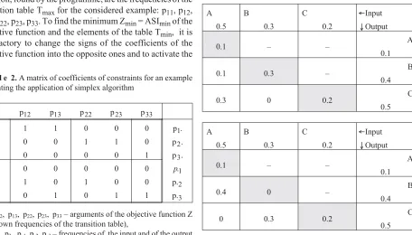
As a result of the program action, the maximum of the objective function as well as the sought values of the varia-bles of the objective function for which the maximum occurs are obtained. In reference to the considered example, Zmax=
ASImax is possibly the highest index of the aggregate
stability, which can be obtained under assigned weights for a given pair of the frequency distributions in the input and in the output. The coefficients of the maximum of the objective function, found by the programme, are the frequencies of the transition table Tmaxfor the considered example: p11, p12,
p13, p22, p23, p33. To find the minimum Zmin= ASIminof the
objective function and the elements of the table Tmin, it is
satisfactory to change the signs of the coefficients of the objective function into the opposite ones and to activate the
programme. For the described example, the following va-lues were obtained:ASImax= 61.3 and ASImin= 37.0. The
respective tables Tmaxand Tminhave the form presented in
Table 3.
The existence of feasible solutions
If the solutions of a problem are sought, first, the issue of its solvability and then the problem of the existence of any feasible solutions should be decided. The considerations pe-rformed till now, as well as the presented examples show, that the problem of finding the extreme transition tables is solvable. The second problem can be reduced to the exami-nation, if for each of any pairs of distributions, a transition table (even if it is just one table) can be constructed. It turns out, that a positive answer exists only for bidirectional chan-ges. Therefore, in case of unidirectional changes, not each pair of distributions can be a distribution of the input and the output. For instance, when k = 2, a pair of distributions [0.4, 0.6] and [0.5, 0.5] cannot, respectively, create the input and the output distributions (under the assumption of destructive direction of aggregates changes). The same pair of distribu-tions for bidirectional changes makes it possible to build lots of transition tables. However, just by changing the roles of these distributions, one can become convinced that in this case for unidirectional changes the only possible transition table is a table with elements: p11= 0.4, p12= 0.1 and p22= 0.5. It is
p11 p12 p13 p22 p23 p33
1 1 1 0 0 0 p1.
0 0 0 1 1 0 p2.
0 0 0 0 0 1 p3.
1 0 0 0 0 0 p.1
0 1 0 1 0 0 p.2
0 0 1 0 1 1 p.3
p11, p12, p13, p22, p23, p33– arguments of the objective function Z
(unknown frequencies of the transition table),
p1., p2., p3., p.1, p.2, p.3– frequencies of the input and of the output
distributions, respectively.
T a b l e 2.A matrix of coefficients of constraints for an example presenting the application of simplex algorithm
A B C ¬Input
0.5 0.3 0.2 ¯Output
0.1 – – A
0.1
0.1 0.3 – B
0.4
0.3 0 0.2 C
0.5
A B C ¬Input
0.5 0.3 0.2 ¯Output
0.1 – – A
0.1
0.4 0 – B
0.4
0 0.3 0.2 C
0.5 Explanations as in Table 1.
T a b l e 3.Extreme transition tables, referring to the example
because, always for k = 2 in case of unidirectional changes, only one transition table exists.
In fact, the problem of the existence of feasible solu-tions is just an academic problem. Because, if the distribu-tions in the input and in the output are the results of testing the aggregates of a soil sample, at least one feasble transition table exists – it is a table Ttest.
Uniqueness of extreme solutions
In case of unidirectional changes for a given pair of fre-quency distributions in the input and in the output, under the presented in this paper criterion of quality changes (thus under the same objective function), if a pair of extreme tran-sition tables and a pair of extreme indices of stability exist, these are the only pairs. It is assured by a specific triangular construction of transition tables and by a selected set of weights. However, the same extreme transition tables can be obtained for different sets of weights, i.e., for different forms of the objective function.
If the results of the action of a destructive factor are uni-directional changes, usually many transition tables can be built for a specific pair of frequency distributions in the input and in the output. The existence of at least one transition table is guaranteed by a performed experiment and by a table Ttest, which is assigned basing on it. Only one transition table exists, when the input and the output distributions are identical or when one of these distributions is reduced to one class. It is obvious, that in this case the extreme indices of stability ASImax, ASIminand ASItestpossess the same value.
CONCLUSION
The simplex algorithm of the linear programming is an effective tool to find the range of extreme indices of the soil aggregates stability of a tested soil sample, both for unidirec-tional and bidirecunidirec-tional models of the aggregate changes.
REFERENCES
1.Braunack M.V. and Dexter A.R., 1989.Soil aggregation in seedbed: a review. I. Properties of aggregates and beds of ag-gregates. Soil Till. Res., 14, 259–279.
2.Childress R.L., 1974.Mathematics for Managerial Decision. Prentice Hall. Inc. New Yersey: Englewood Cliffs.
3.Czerwiñski Z., 1983.Mathematics in Economy (in Polish). PWN, Warszawa.
4.Dexter A.R., 1988. Advances in characterization of soil stru-cture. Soil Till. Res., 11, 199–238.
5.Feller W., 1961.An Introduction to Probability Theory and its Applications. Wiley and Sons, New York.
6.Góralski A., 1987.Description Methods and Statictic Conclu-sions in Psychology and Pedagogics (in Polish). PWN, Warszawa. 7.Hillel D., 1998.Environmental Soil Physics. Academic Press,
London.
8.Hillier F.S. and Lieberman G.J., 1986. Introduction to Operations Research. 4th Edition. Mc Graw Hill, New York. 9.Ignasiak E. (Ed.), 2001.Operations Research (in Polish).
PWN, Warszawa.
10.Niewczas J. and Witkowska-Walczak B., 2003.Index of ag-gregates stability as linear function value of transition matrix elements. Soil Till. Res., 70/2, 121–130.