The Wavelet Transform-Domain LMS Adaptive Filter Algorithm with Variable Step-Size

1. Introduction

Adaptive filters are widely used in various applications such as system identification, channel equalization, noise cancellation, active noise control, and so on [1], [2]. The most popular adaptive filters are the least mean squares (LMS) and normalized LMS (NLMS) algorithms due to their simplicity. However, these algorithms have slow convergence for colored input signals [3], [4]. To solve this problem, the transform domain adaptive filter (TDAF) algorithms have been proposed [5].

The TDAF algorithms exploit the de-correlation proper-ties of some well-known signal transforms, such as the discrete Fourier transform (DFT) and the discrete cosine transform (DCT), in order to pre-whiten the input data and speed up filter convergence [6], [7], and [8]. In the wavelet transform domain least mean square (WTDLMS) adaptive filtering, the projections of the input signal onto the orthogonal subspaces are used as inputs to a linear combiner. The weights of the linear combiner can hence be updated by the LMS algorithm while normalizing the power at each resolution level to achieve faster and uni-form convergence of all weights to the optimal [9], [10].

In the above mentioned algorithms, the fixed step-size can change the convergence rate and the steady state mean square error (MSE). With optimally selecting the step-size during the adaptation, we obtain fast convergence rate and low steady state mean square error at the same time. In the case of variable step-size (VSS) methods, various ap-proaches have been proposed in the literatures [11], [12]. One of the most important strategy in this issue was

pre-The Wavelet Transform-Domain LMS Adaptive Filter

Al-gorithm with Variable Step-Size

M. Shams Esfand Abadi*(C.A.), H. Mesgarani*and S. M. Khademiyan*

Abstract:The wavelet transform-domain least-mean square (WTDLMS) algorithm uses the

self-orthogo-nalizing technique to improve the convergence performance of LMS. In WTDLMS algorithm, the trade-off between the steady-state error and the convergence rate is obtained by the fixed step-size. In this paper, the WTDLMS adaptive algorithm with variable step-size (VSS) is established. The step-size in each subfilter changes according to the largest decrease in mean square deviation. The simulation results show that the proposed VSS-WTDLMS has faster convergence rate and lower misadjustment than ordinary WTDLMS.

Keywords:Adaptive Filter, Wavelet Transform Domain LMS (WTDLMS), Variable Step-Size, Mean Square

Deviation

Iranian Journal of Electrical & Electronic Engineering, 2017. Paper first received 25 December 2016 and accepted 11 July 2017. * The Author is with the Faculty of Electrical Engineering, Shahid Ra-jaee Teacher Training University, P.O.Box: 16785-163, Tehran, Iran. Emails: [email protected]

** The Authors are with the Faculty of Basic Sciences, Department of Applied Mathematics, Shahid Rajaee Teacher Training University, P.O.Box 16785-163, Tehran, Iran.

Emails: [email protected], [email protected]

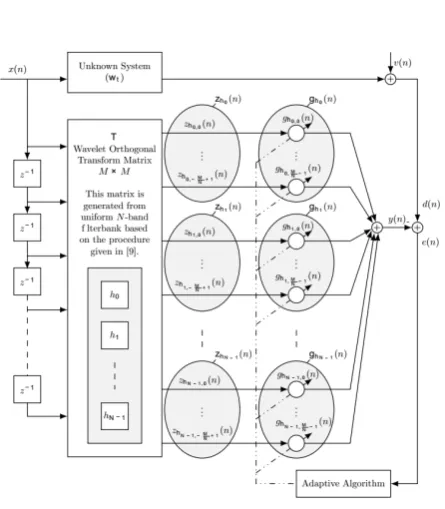
Corresponding author: M. Shams Esfand Abadi Fig. 1.Structure of the WTDLMS algorithm.

sented in [13]. This approach was successfully extended to the different adaptive filter algorithms in [14]. In this paper, the VSS-WTDLMS is introduced. In the proposed VSS-WTDLMS, the step-size in each subfilter changes according to the largest decrease in mean square devia-tion. In comparison with ordinary WTDLMS [15], the VSS-WTDLMS has faster convergence speed and lower steady-state MSE.

The reminder of this paper is organized as follows. In Sec-tion 2, the WTDLMS algorithm is briefly reviewed. The new VSS-WTDLMS is proposed in Section 3. The com-putational complexity of the VSS-WTDLMS is discussed in Section 4. Finally, before concluding the paper, the use-fulness of this algorithm is demonstrated by presenting several simulation results.

Throughout the paper, represents transpose, takes the squared Euclidean norm, and shows the Expectation.

2. The WTDLMS Adaptive Algorithm Consider a linear data model for as

(1)

where w_tis an unknown M-dimensional vector that we expect to estimate, υ(n)is the measurement noise with-variance σ2

υ, and

denotes an M-dimensional input (regressor) vector. It is assumed that υ(n) is zero mean, white, Gaussian, and independent of x(n). Fig. 1 shows the structure of the WTDLMS algo-rithm [9]. In this figure, the MxMmatrix T is an orthogo-nal matrix that is derived from a uniform N-band filter bank with filters denoted by h₀, h₁, ..., h_N-1following the procedure given in [9]. In matrix form, the orthogonal WT can be expressed as z(n)=Tx(n). This vector can be

rep-resented as where ’s

are output vectors of an N-band filter bank. By splitting the g(n)into N subfilters, each having coefficients, , the output signal can be stated as

(2)

and the error signal is obtained by . The update equation for each subfilter in WTDLMS is given by

(3)

where can be computed iteratively by

(4)

with a smoothing factor .

3. The VSS-WTDLMS Adaptive Algorithm

By defining the weight error vector , where is the true unknown subfilter coefficients, the weight error vector update equation for WTDLMS for each subfilter can be represented as

(5)

In (5), is a variable step-size in subfilter. Taking the squared Euclidean norm from the both sides of (5) and then the expectation leads to

(6)

where

(7)

Maximizing Δ with respect to leads to the follow-ing optimum step-size

(8)

Since , we use the approximation

for a priori error as, .

Therefore we have

(9)

By defining , we obtain that

. Then, the optimum step-size is

given by ( ) T( ) _t ( )

d n x n w X n

1 0 ( ) ( ) ( ) i i N T h h i

y n n n

¦

( )n [ ( ), (x n x n1),}, (x n M 1)]T

x

0 1 1

( ) [ ( ), ( ), , ( )] N

T T T T

h h h

n n n } n

z z z z ( )

i

h n

z

M N

0 1 1

( ) [ ( ), ( ), , ( )] N

T T T T

h h h

n n n } n

g g g g

( )n ( )n ( )

e d y n

2 ( )

( 1) ( ) ( )

( ) i i i i h h h h n

n n n

n e P V z g g 2 ( ) i h n V 2 2 2

( ) ( 1) (1 ) ( )

i i i

h n h n h n

V DV D z

D D

( ) ( )

i i i

h n h h n

g g$ g

i

h g$

2 ( )

( 1) ( ) ( ) ( )

( ) i

i i i

i

h

h h h

h

e n

n n n n

n P

V

z

g g

2 2

[ ( 1) ] [ ( ) ]

i i

h h

E g n E g n '

2 2 2 4 2 ( ) ( ) ( )

2 ( ) [ ]

( ) ( ) ( ) ( ) [ ] ( ) i i i i i i i T h h h h h h h

n n n

n E n n n n E n e e P V P V ' g z z ( ) i h n P ( ) i h n P 2 2 4 2 ( ) ( ) ( ) [ ] ( ) ( ) ( ) ( ) [ ] ( ) i i i i i i T h h h h h h

n n n E n n n n E n e e V P V g z z $ 2 2 2 2 2 4 4 2 ( ) [ ] ( ) 1 ( ) ( ) ( ) ( ) [ ] [ ] ( ) ( ) i i i i i i h h h a h h h a n E n n

N _{n n n}

E E e n n e X V P V V V | z z $ 1 0 ( ) ( ) ( ) i i N T

a i h h

e n

_¦

( ) ( ) ( )

i i

T

a h h

e n Ng n z n

2

( ) ( )

( )

( ) hi a

i _hi

n e n

h n V _n

z q 2 2 4 2 ( ) ( ) ( ) ( ) i i i h h a h

e n n n

n V

z

q

(10)

Applying the expectation into the leads to the

(11)

We propose to estimate by time averaging as follows:

(12)

where . Using instead of ,

the VSS-WTDLMS for each subfilter is established as

(13)

where

(14)

The fully update equation for VSS-WTDLMS can be ex-pressed as

(15)

Where

(16)

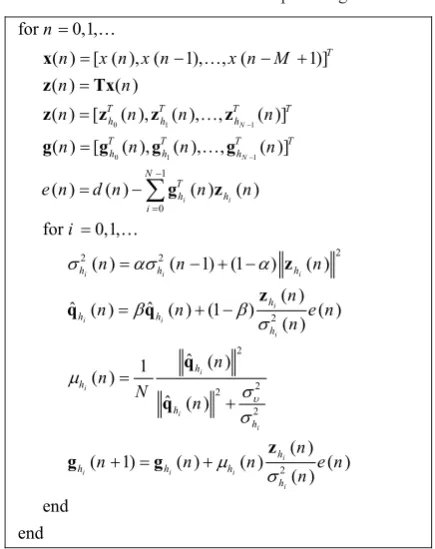
and is the matrix. Table 1 summa-rizes the procedure of the VSS-WTDLMS adaptive algo-rithm.

4. Computational Complexity

Table 2 describes the computational complexity of the proposed VSS-WTDLMS algorithm. The number of mul-tiplications and divisions have been calculated for each terms. In the following, Table 3 compares the computa-tional complexity of various VSS-TDLMS algorithms. These algorithms are from [7], [11], [12] and [14]. In this Table, Mis the number of filter coefficients, Nis the

num-ber of subbands, M_iis the number of past values of the ith transform coefficient, and Lis number of past squared val-ues of the error. The VSS-WTDLMS algorithm needs M2_{+6M+5N multiplications and 4Ndivisions. It is}

inter-esting to note that using Haar wavelet transform (HWT) leads to the only 6M+5Nmultiplications which is signif-icantly lower than other VSS transform domain adaptive algorithms.

5. Simulation Results

We demonstrated the performance of the proposed algo-rithm by several computer simulations in a system iden-tification scenario. The unknown impulse response is randomly selected with 16 taps (M=16). The input signal is an AR(1) signal generated by passing a zero-mean white Gaussian noise through a first-order system . An additive white Gaussian noise was added to the system output, setting the signal-to-noise ratio (SNR) to 30 dB. The Haar wavelet transform (HWT) was used in all simulations which leads to the reduction of computational complexity due to the elements (+1 and -1) in HWT. The values of α and β were set to 0.995 and 0.9 respectively. 2 2 2 ₂ 4 [ ( ) ] 1 ( ) ( ) [ ( ) ] [ ] ( ) i i i i i h h h h h E n n N _n

E n E n X P V V | q z q $ 2 ( ) ( ) [ ( )] [ ] ( ) i i i h h h n n e n E n E

V

z

q

2 ( ) ( )

ˆ ( ) ˆ ( ) (1 )

( ) i i i i h h h h e n n n n n E E V z q q [ ( )] i h E q n

2 ( )

( 1) ( ) ( ) ( )

( ) i

i i i

i h

h h h

h

n

n n n n

n e P

V

z

g g

0 E 1

2

ˆ ( ) i

h n

q [ ( )2]

i h

E q n

2

2 2

2

ˆ ( ) 1

( )

ˆ ( )

i i i i h h h h n n N n X P V V | q q 0 1 1

( ) 0 0

0 ( ) 0

( )

0 0 ( )

N h h h n n n n § · ¨ ¸ ¨ ¸ ¨ ¸ ¨ ¸ ¨ ¸ © ¹ C C C C

(n1) ( )n ( ) ( ) ( )n nen

g g C z

2

( )

( )

( ) hi .

i _hi

n

h n n

P

V

C I M M

NuN

1 1 1 0.9 ( ) z H z

0 1 1

0 1 1

1

0

2

2 2

for 0,1,

( ) [ ( ), ( 1), , ( 1)]

( ) [ ( ), ( ), , ( )] ( ) [ ( ), ( ), , ( )] ( ) ( ) ( ) ( ) for 0,1, ( ) ( ) (

( 1) (1 ) ( )

( ) ˆ ) N N i i

i i i

i

T

T T T T

h h h

T T T T

h h h

N T

h h

i

h h h

h

n

n x n x n x n M

n n n n

n n

n n n

n n n n

i

n n n

n n

e d

V DV D

} } }

_¦

z z z z

g g g g

g z z q z Tx 2 2 2 2 2 2 ( )

ˆ ( ) (1 ) ( )

( )

ˆ ( ) 1

( )

ˆ ( )

( )

( 1) ( ) ( ) ( )

( ) end end i i i i i i i i

i i i

i h h h h h h h h

h h h

h n n n n n n N n n

n n n e n

n e X E E V P V V P V z q q q z g g

Table 1.The VSS-WTDLMS Adaptive Algorithm.

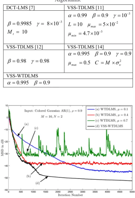
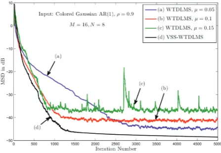
Figs. 2-4 show the mean square deviation (MSD) learning curves of proposed VSS-WTDLMS and ordinary WT-DLMS algorithm for different values of N. In WTDLMS, different values for the step-size have been selected. We observe that VSS-WTDLMS has faster convergence speed and lower steady-state error than ordinary WT-DLMS algorithm for all values of N. The comparison of VSS-WTDLMS with recently and famous VSS-TDLMS algorithms has been presented in Fig. 5 [7], [11], [12] and [14]. The parameters of the simulated algorithms have been chosen according to the Table 4. This figure shows that, the proposed VSS-WTDLMS has better convergence speed an lower steady-state error than other VSS-TDLMS algorithms for all values of N. Also, the computational complexity of the proposed algorithm is lower than other

Equation insubband Total

u y u y

( )n ( )n

z Tx - - 2

M

-( ) ( )n T( ) ( )

e n d g n z n - - M

-2 2 2

( ) ( 1) (1 ) ( )

i i i

h n h n h n

V DV D z M 2

N - M 2N

-2

( )

ˆ ( ) ˆ ( ) (1 ) ( )

( ) i

i i

i

h h h

h

n

n n e n

n

E E

V

z

q q 2M 1

N 1 2M N N

2

2 2

2

ˆ ( ) 1

( )

ˆ ( ) i

i

i

i

h h

h

h

n n

N

n X

P

V V

q

q 1

M

N 2 M N

2N

2

( )

( 1) ( ) ( ) ( )

( ) i

i i i

i

h h h h

h

n

n n n n

n e

P V

z

g g M 1

N 1 M N N

Total Multiplications: M26M 5N

Table 2.The Computational Complexity of VSS-WTDLMS Algorithm

Algorithm Multiplications Divisions

DCT-LMS [7] 2

+4 1

( _t )

M M M 2M

VSS-TDLMS [11] 2

5 2

M M L M 1

VSS-TDLMS [12] 2

8 8

M M M 1

VSS-TDLMS [14] 2

5 8

M M M 1

VSS-WTDLMS 2

6 5

M M N 4N

VSS-WTDLMS

(HWT) 6M 5N

4N Table 3.The Computational Complexity of Various

VSS-WTLMS

DCT-LMS [7] VSS-TDLMS [11]

3

0.9985 8 10

10

t M

E J

u

3

2

3

0.99 0.9 10

10 5 10

4.7 10 max

min

L μ

μ

D E J

u u

VSS-TDLMS [12] VSS-TDLMS [14]

0.98 0.98

E J 2

0.995 0.9 0.9

0.5 max

μ C M X

D E J

V u

VSS-WTDLMS

0.995 0.9

D E

Table 4.The Parameters In VSS-TDLMS and VSS-WTDLMS Algorithms.

Fig. 2.The MSD learning curves of WTDLMS and VSS-WT-DLMS algorithms with N = 2.

VSS-TDLMS algorithms due to using HWT.

Fig. 6 presents the variation of the step-size in each sub-band for VSS-WTDLMS algorithm during the adaptation. As we can see, the step-sizes start from large values and end with low values for N=2, 4, and 8. Finally, Fig. 7 shows the number of filter coefficients versus the filter length for VSS-TDLMS, WTDLMS, and VSS-WTDLMS algorithms. This figure indicates that the computational complexity of VSS-WTDLMS with HWT is significantly lower than other algorithms.

6. Conclusion

In this paper, the WTDLMS with VSS was established. The step-size in each subband changes according to the largest decrease in mean square deviation. The simulation results indicated that the proposed VSS-WTDLMS had Fig. 3.The MSD learning curves of WTDLMS and

VSS-WT-DLMS algorithms with N = 4.

Fig. 4.The MSD learning curves of WTDLMS and VSS-WT-DLMS algorithms with N = 8.

Fig. 5.The MSD learning curves of various VSS-TDLMS and VSS-WTDLMS algorithms.

Fig. 6.Variation of the step-size in each subband during the adaptation for VSS-WTDLMS.

Fig. 7.The number of filter coefficients versus the filter length (M) in various TDLMS, WTDLMS, and

VSS-WTDLMS algorithms.

faster convergence speed and lower steady-state error than ordinary WTDLMS and other VSS-TDLMS algorithms. Also, the computational complexity of VSS-WTDLMS with HWT was significantly lower than other algorithms.

References

[1] B. Widrow and S. D. Stearns, "Adaptive Signal Processing". Englewood Cliffs, NJ: Prentice-Hall, 1985.

[2] S. Haykin, “Adaptive Filter Theory”. NJ: Prentice-Hall, 4th edition, 2002.

[3] B. Farhang-Boroujeny, “Adaptive Filters: Theory and Applications”. Wiley, 1998.

[4] A. H. Sayed, “Fundamentals of Adaptive Filter-ing”. Wiley, 2003.

[5] A. H. Sayed, “Adaptive Filters”, Wiley, 2008. [6] S. S. Narayan, A. M. Peterson, and M. J.

Narashima, “Transform domain LMS algorithm,” IEEE Trans. Acoust., Speech, Signal Processing, vol. ASSP-31, pp. 609–615, 1983.

[7] D. I. Kim and P. D. Wilde, “Performance analysis of the DCT-LMS adaptive filtering algorithm,” Sig-nal Processing, vol. 80, pp. 1629–1645, Aug. 2000. [8] S. Zhao, Z. Man, S. Khoo, and H. Wu, “Stability and convergence analysis of transform-domain LMS adaptive filters with second-order autoregres-sive process,” IEEE Trans. Signal Processing, vol. 57, pp. 119–130, Jan. 2009.

[9] S. Attallah, “The wavelet transform-domain LMS algorithm: a more practical approach,” IEEE Trans. Circuits, Syst. II: Analog and Digital Signal Processing, vol. 47, no. 3, pp. 209–213, Mar. 2000. [10] S. Attallah, “The wavelet transform-domain LMS adaptive filter with partial subband-coefficient up-dating,” IEEE Trans. Circuits, Syst. II: EXPRESS BRIEFS, vol. 53, no. 1, pp. 8–12, Jan. 2006. [11] R. Bilcu, P. Kuosmnen, and K. Egiazarian, “A

transform domain LMS adaptive filter with variable step size,” IEEE Signal Processing Letters, vol. 2, pp. 51–53, Feb. 2002.

[12] K. Mayyas, “A transform domain LMS algorithm with an adaptive step size equation,” in Proc. IS-SPIT, Rome, Italy, 2004, pp. 28–30.

[13] H. C. Shin, A. H. Sayed, and W. J. Song, “Variable step-size NLMS and affine projection algorithms,” IEEE Signal Processing Letters, vol. 11, pp. 132– 135, Feb. 2004.

[14] S. Zhao, D. L. Jones, S. Khoo, and Z. Man, “New variable step-sizes minimizing mean-square devia-tion for the LMS-type algorithms,” Circuits, Sys-tems, and Signal Processing, vol. 33, pp. 2251–2265, 2014.

[15] M. Shams Esfand Abadi, H. Mesgarani, and S. M. Khademiyan. "The Wavelet Transform-Domain LMS Adaptive Filter Employing Dynamic Selection

of Subband-Coefficients." Digital Signal Process-ing, vol. 69, pp. 94-105, Oct. 2017.

M. Shams Esfand Abadi re-ceived the B.S. degree in Electrical Engineering from Mazandaran University, Mazandaran, Iran and the M.S. degree in Electrical En-gineering from Tarbiat Modarres University, Tehran, Iran in 2000 and 2002, re-spectively, and the Ph.D. degree in Biomedical En-gineering from Tarbiat Modarres University, Tehran, Iran in 2007. Since 2004 he has been with the Department of Electrical Engineering, Shahid Rajaee University, Tehran, Iran, where he is cur-rently an associate professor. His research interests include digital filter theory, adaptive distributed networks, and adaptive signal processing algo-rithms.

H. Mesgarani received the M.Sc. and Ph.D. degrees in applied mathematics from Iran University of Science and Technology, Tehran, Iran, in 1996 and 2002, respectively. He is an Associate Professor with the Department of Math-ematics at the Shahid Rajaee Teacher Training University, Tehran, Iran. He joined the Department in 2002. His research inter-ests include Integral equations and Wavelet func-tions.

S. M. Khademiyan received the M.Sc. degree in applied mathematics from Iran Uni-versity of Science and Tech-nology, Tehran, Iran, in 2012. Currently, he is a Ph.D. can-didate at the Department of Mathematics, Faculty of Sci-ence, Shahid Rajaee Teacher Training University, Tehran, Iran. His research in-terests include digital filter theory and adaptive sig-nal processing algorithms.