Modelling and Decision-making on Deteriorating Production Systems using Stochastic Dynamic Programming Approach

Please cite this article as: S. Yazdanparast, A. Sadegheih, M. Fallahnezhad, M. Abooie, Modelling and Decision-making on Deteriorating Production Systems using Stochastic Dynamic Programming Approach, International Journal of Engineering (IJE), IJE TRANSACTIONS C: Aspects Vol. 31, No. 12, (December 2018) 2052-2058

International Journal of Engineering

Modelling and Decision-making on Deteriorating Production Systems using

Stochastic Dynamic Programming Approach

S. Yazdanparast, A. Sadegheih*, M. Fallahnezhad, M. Abooie

Department of Industrial Engineering, Yazd University, Yazd, Iran

P A P E R I N F O

Paper history:

Received 26 May 2018

Received in revised form 15 September 2018 Accepted 26 October 2018

Keywords:

Machine Replacement

Stochastic Dynamic Programming Stochastic Deterioration

A B S T R A C T

This study aimed at presenting a method for formulating optimal production, repair and replacement policies. The system was based on the production rate of defective parts and machine repairs and then was set up to optimize maintenance activities and related costs. The machine is either repaired or replaced. The machine is changed completely in the replacement process, but the production rate of defective parts decreases in the repair process. The repair time and number of repairs will affect this process. The aim of this study is to find decision variables that minimize the final cost of repair, replacement, maintenance and prevention of failures in a given time horizon. As a case study, the variables were evaluated at Arak Pishgam Company to achieve optimal conditions. The proposed model was developed based on the semi-Markov decision process (SMDP). In addition, stochastic dynamic programming model was used to achieve optimal conditions.

doi:10.5829/ije.2018.31.12c.09

1. INTRODUCTION

1

There is a need for a more detailed study on the relationship between the factors affecting the performance of production systems, in particular, the interactions of productivity, quality (repair/replacement) and the design of industrial production systems. Unfortunately, there are not enough models or instructions or at least basic principles which consider all these factors and their impact. Only primary experience and research indicate that product design determines the major part of product quality (repair/replacement). However, the quality of parts can still be affected by the production process. Therefore, there is an interaction between production and repair/replacement [1]. The use of effective preventive maintenance strategies will significantly increase the value added of production activities. Accordingly, maintenance is used as a globally accepted principle in manufacturing institutions.

*Corresponding Author Email: [email protected] (A. Sadegheih)

2. LITERATURE REVIEW

The first studies in this area, such as Reichel’s paper, include stochastic uncertainty. Therefore, this article is an important contribution, because it provides optimal conditions to obtain the optimal strategy [5]. Subsequently, Olsder and Suri introduced a dynamic programming model in which machine failures are repaired according to a well-known Markov process. They set up a feedback control of the routing portions of the machine which minimizes the time to complete a specific production objective. These models are an important source for understanding required parameters for determining optimal production control policies for unsteady production systems [1]. In this regard, a few studies [6] are also of great importance, because they provided a hierarchical control algorithm in which the production management problem involves compliance with production requirements while the machine failures are repaired at random times. This research work and related articles investigated system dynamics, cost structure, and variables and thus are usually used as most-cited references in this field [6]. Deterioration of a machine at a risk of failure has attracted attention of various researchers who proposed a repair/replacement policy [7]. Their model represents whether it is easy to repair a machine in failure or it is better to replace the machine. They assumed that the severity of failure depends on the age of machine. Nevertheless, they did not consider production decisions in their model [7].

In another study, Lai and Chen [8] analyzed optimal replacement policy of a two-unit system with failure rate interaction between the units. This interaction implies that when the first machine fails, a certain damage is imposed to the second machine and when the second unit fails, the first machine instantly fails. In addition, machine failure rate also increases due to deterioration [6-8]. Wu and Clement-Chroome [9] proposed a model for a repairable system for cases where one or two maintenance policies are implemented. Their model provides details on estimation of the value of required parameters. Furthermore, their method allows modeling of different phases of deterioration during system lifetime by focusing on the failure severity [9]. Fallahnejad and Pourgharib [10-12] proposed a maintenance policy plan for machine replacement as a maintenance model considering the quality of manufactured parts. For this purpose, a decision tree was developed for maintenance on a finite time horizon based on the sequence sampling which includes replacement (Renew) and production continuation (Do nothing) decisions. Consequently, they reached an optimal decision threshold to minimize expected cost [10-11]. In another study, the optimal machine replacement policy was proposed based on the production rate of defective parts. The aim was to make

the optimal decision using Markov decision process (MDP). Production and repair costs were considered in the model. The machine cost was also considered at the end of the period. In each interval, decision must be taken on production or repair on the basis of maximum profitability [4-12].

3. PRODUCTION SYSTEMS

Stochastic control has been recently widely used and studied, because it offers an interesting approach which allows for taking into account uncertainty in the dynamics of production systems.

In a real production system, defective parts may be produced at a given rate. Consequently, if a machine gradually fails due to combined effects of erosion, aging, deterioration, imperfect repairs, etc., the production rate of defective parts can be strongly influenced by deterioration [13]. Based on the above discussion, one can claim that an integrated model is required for providing more details on the relationship between quality aspects (repair/replacement) and production management. This integrated model will explain how this interaction can be influenced by other phenomena such as deterioration and how maintenance strategies can be determined to deal with problems

.

3. 1. Optimal Policies Considering Deterioration

A system will be repaired when it fails or reaches to a certain operation time. A machine is replaced with a new machine after a certain number of failures. Deterioration requires a decrease in the operation time after repair while increasing number of repairs after failure. In addition, they introduced a lifetime distribution considering the effects of maintenance and repair activities [14-15]. According to the above-mentioned studies, one can conclude that none of the papers have paid attention to this fact about deteriorating systems that deterioration can also affect the quality of produced parts or there may be a simultaneous effect on the quality and other machinery parameters. Furthermore, considering the relationship between deterioration and quality, preventive maintenance can also play an active role in the optimal control policy. Extreme competition with advanced and growing technology has made considerable changes in the industrial perspective. New products, processes and systems are constantly being developed and exploited. For this reason, the levels of equipment utilization should be improved through observing correct programs.

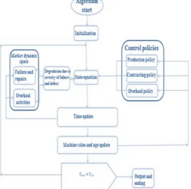
simulation method is provided which combines a simulation model and statistical analysis. This method has been used in several studies [16] and includes the following steps (see Figure 1):

Step 1: Control problem formulation In this step, the formulas of the stochastic dynamic programming model for a production system are analyzed to determine system dynamics, different modes of the system and average expected cost.

Step 2: The structure of optimal control policies

Numerical methods are used to approximate the structure of control policies. Accordingly, the control parameters (Z0, SA, A, B) are determined.

Step 3: Simulation model A simulation model is used for constructing the accurate stochastic behavior and all features of the production system. The simulation model uses the control parameters as inputs to evaluate the system performance and total costs as outputs.

Step 4: Statistical analysis Through a series of simulated outputs, statistical analysis is used to identify how changes in control parameters can be used to determine the main factors and their interactions.

Step 5: Parameter optimization Upon identifying the main factors and the relationships between them, the response surface methodology (RSM) is used to determine the relationship between the main factors and the total expected cost. In summary, the results of the sensitivity analysis emphasize the complex interaction between production, contractors and machinery deterioration.

4. SIMULATION MODEL

This section pays attention to a simulation model as shown in Figure 1in order to solve research issue.

Figure 1. Simulation algorithm of studied model

The model includes a number of networks which describe a particular activity or occurrence of an event in system. These networks are as follows:

1. Initialization: This section determined various values of parameters such as control parameters

(

)

(

)

transition values for different modes. Furthermore, it defines simulation time and also necessary time for system to reach steady state.

2. Failure and repair: This section models Markov essential and dynamic failure and repairs. Therefore, it uses transition values of previous section. This section connects "state equation" block in order to define the failure or operational status.

3. Production control policy: These policies are defined to explain appropriate production rate according to stock level and machine age. A set of labels are used in this section to determine when the current stock level or machine age reaches a certain level, and then the production rate is determined.

4. Subcontracting policy: Using an inspection mechanism, the stock level and machine age are permanently monitored.

5. Overhaul policy: This section is related to repair and failure block in order to be coordinated with stochastic events (including defect, repair and overhaul). This block is also interacting with "state equation" block in order to fix rates of failures and defects which have already been overhauled.

6. Degradation block: It uses data from failure and repair block, production, subcontracting policies and overhaul to update failure rates and severity of failures as described earlier. Effects of decline almost take back to initial conditions when overhauling is done.

7. State equation: It is one of the most important model components which determine stock level and machine age. For proper function, there is a need for information about production rate, failure rate, machine status, overhaul, subcontracting rate, etc. Furthermore, this block interacts with several other blocks of model.

8. Advance time: Current time is updated by combination of timing discrete events (such as defects, repair and overhaul), continuous variables (such as stock level or machine age) and characteristics of time steps.

9. Update stock and age level: This block tracks any changes in stock levels and machine age, and estimates cumulative values of variables using Runge-Kutta-Fehlberg algorithm.

At the end of simulation process, the expected total cost J(.) is calculated by Equation (7). During of TSim simulation is defined for hundred thousand time units to stabilize system stability.

5. NUMERICAL MODEL SOLUTION

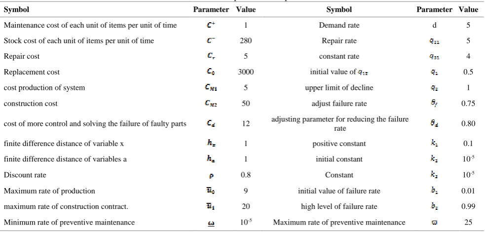
In this section, we use numerical method for determining optimal control policies based on Kushner's method. Application of an approximate design for value function gradient is the main idea of this method. Table 1presents applied parameters for instance the numerical ones:

In this section, we combine simulation model with statistical analysis based on designed tests and optimized parameters by response surface method. Stock level and

machinery age are approximated to determine control parameters.

Figure above is designed in order to facilitate estimation of control parameters. Stock level represents Z0, and point B represents production. SA point defines overhaul policy. Point A is defined to determine contracting policy. We can control production system and estimate the entire possible cost by approximation of these parameters.

Analysis of variance (ANOVA) is applied to analyze simulated data. Therefore, we used a dependent variable (total possible cost) and three independent variables (Z0, SA, B). Simulation was repeated 108 times.

Table 2 presents applied costs for statistical analyses. Table 3 shows Factor levels for statistical analysis.

TABLE1. Example numerical parameters

Symbol Parameter Value Symbol Parameter Value

Maintenance cost of each unit of items per unit of time 1 Demand rate d 5

Stock cost of each unit of items per unit of time 280 Repair rate 5

Repair cost 5 constant rate 4

Replacement cost 3000 initial value of 0.5

cost production of system 5 upper limit of decline 1

construction cost 50 adjust failure rate 0.75

cost of more control and solving the failure of faulty parts 12 adjusting parameter for reducing the failure

rate 0.80

finite difference distance of variable x 1 positive constant 0.1

finite difference distance of variables a 1 initial constant 10-5

Discount rate 0.8 Constant 10-5

Maximum rate of production 9 initial value of failure rate 0.01

maximum rate of construction contract. 20 high level of failure rate 0.99

Minimum rate of preventive maintenance 10-5 _{Maximum rate of preventive maintenance 25}

TABLE2.Cost parameters for statistical analysis

Parameter C+ C- CM1 CM2 C0 Cd

Value 1 280 5 50 3000 12

TABLE3.Factor levels for statistical analysis

Description High

level Medium

Low

level Factors

Machinery production

threshold 8 5 2 Z0

Necessary machine age

for complete overhaul 50 40 20 SA

Age limit to stop machine 75 60 45 B

Table 4 shows the results of ANOVA. R2 value of model is estimated equal to 0.87. This parameter indicates that 87% of changes in total possible cost variable can be interpreted by independent variables of model, and this indicates high power of model. Furthermore, direct and mutual effects of three independent variables are significant at confidence level of 95%.

6. RESULT SENSITIVITY ANALYSIS

TABLE4.ANOVAresults for total cost variable

Variable Sum of error

square Degrees of freedom F statistics P-value

A: Z0 83.33 1 19.22 0.0007

B: SA 1787 1 1892.09 0.0000

C: B 197.34 1 64.33 0.0000

AA 52.98 1 18.91 0.0005

AB 87.98 1 23.87 0.0000

AC 88.09 1 81.10 0.0009

BB 3401.22 1 1002.19 0.0000

BC 40.92 1 23.87 0.0108

CC 302.22 1 102.39 0.0000

Blocks 9.34 3 1.92 0.8500

Total error 629.04 95

Total (corr.) 3109.23 107

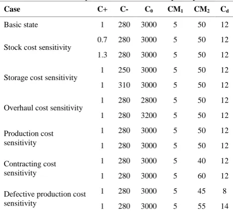
Table 5 presents seven states of cost parameters derived from original state. In this section, we investigate effects of these parameters on control parameters and total incurred costs.

Set of cost value includes costs associated with stock, storage, overhaul, defective products, production, and contracting costs. Results of sensitivity analysis are presented in Table 6. This table shows relationship between changes in cost and control parameters and its costs.

Changes in stock cost parameter (C+_{): An increase}

unit in c+ _{will lead to reduced three control parameters}

because high c+ _{will reduce stock level more than Z} 0

value.

TABLE5.Cost parameters for sensitivity analysis

Case C+ C- C0 CM1 CM2 Cd

Basic state 1 280 3000 5 50 12

Stock cost sensitivity

0.7 280 3000 5 50 12

1.3 280 3000 5 50 12

Storage cost sensitivity 1 250 3000 5 50 12

1 310 3000 5 50 12

Overhaul cost sensitivity 1 280 2800 5 50 12

1 280 3200 5 50 12

Production cost sensitivity

1 280 3000 5 50 12

1 280 3000 5 50 12

Contracting cost sensitivity

1 280 3000 5 40 12

1 280 3000 5 60 12

Defectiveproduction cost sensitivity

1 280 3000 5 45 8

1 280 3000 5 55 14

TABLE6.Analysis of sensitivity of cost parameters

Case Z0* SA* B* Optional _cost Remark

Basic state 5.43 44.72 64.19 68.34 Compared

with baseline

Stock cost sensitivity

7.54 45.90 67.04 66.23 Z1↑, SA↑, B↑,

C↓

4.22 43.54 61.34 70.45 Z1↓, SA ↓, B

↓, C ↑

Storage cost sensitivity

5.13 44.60 63.64 68.14 Z1↓, SA ↔, _{B↓, C↓}

5.73 44.84 64.74 68.54 Z1↑, SA ↔,

B↑, C↑

Overhaul cost sensitivity

4.78 40.70 63.09 66.00 Z1↓, SA ↓,

B↓, C ↓

6.06 48.74 65.29 30.68 Z_{B↑, C ↑} 1↑, SA ↑,

Production cost sensitivity

5.49 45.78 69.30 65.35 Z1↔, SA ↑,

B↑, C↓

5.38 43.66 59.08 71.33 Z1↔, SA ↓,

B↓, C↑

Contracting cost sensitivity

5.00 45.87 66.09 66.04 Z1_{B↑, C↓} ↓, SA ↑,

5.86 43.57 62.29 70.64 Z1↑, SA ↓,

B↓, C ↑ Defective

production cost sensitivity

5.45 46.98 67.39 62.79 Z1↔, SA ↑,

B↑, C↓

5.41 42.46 60.99 73.89 Z1↔, SA ↓, _{B↓, C↑}

Furthermore, reduced threshold will lead to the reduced complete overhaul and then reduced SA and B because machine will reach its maximum rate at the shortest time, and thus the defective rate will be reduced; contractors will commit demand for products before due time, and consequently B-value will be increased.

Changes in storage cost parameter (C-_{): When c}

-value is increased, Z0 will be enhanced because storage

costs of products are increased, so we need more storage for temporary compensation of shortcomings. In addition, the increased parameter B will considerably lead to complete overhaul. Since storage cost will be increased by higher c-_{, machines remain in operational}

state for further time. Based on obtained results of table, effect of storage cost is on the contrary to stock cost.

Changes in complete overhaul parameter (C0): An

increase unit in C0 will lead to increased Z0 threshold

because since the repair activities with higher C0 are

expensive, we need more space for performing complete overhaul.

Changes in production cost (CM1): When production cost is increased, production with machinery will become very expensive, and thus it will lead to a reduction in threshold of Z0 value. However, this higher cost will lead to lower overhaul cost and reduced SA and B point.

Changes in failure cost (CD): When cd is increased, SA and point B values will be reduced to prevent production of defective units.

7. CONCLUSION AND SUGGESTIONS

A general review of various methods for deterioration modeling shows that deterioration only affects the number of successive system operations or repairs. Literature review also showed that there is no study on the interrelationship between deterioration and quality and its effect on control policy. Therefore, the role of deterioration in quality and its impact on control policy were emphasized in this study. This can be considered as innovation of this research work.

The final evaluation of the model and its acceptable results indicate that the simulation approach used in this study enables us to study complex phenomena in real production systems.

The simulation method used in this study allows analysis and optimization of parameters related to control policies through the design of experiments using the response surface methodology.

The stochastic dynamic programming model used in this study can be used in future studies through heuristic algorithm, ideal planning and so on to compare their results with those obtained in this study.

It is recommended that the Arak Pishgam Company reduce the costs of manufacturing and repairs and maintence of machinery based on the paper model and , accordingly, specify the time of replacement or repair of machinery .

8.REFERENCES

1. Rostamian, H., Total Productive Maintenance (TPM) , Termeh Publications. (2008).

2. Hajshirmohammadi, Ali., Total Productive Maintenance (TPM),

Arkan Publications. (2000).

3. Sepanlou, K.,Behzad, M. "Principles and fundamentals of vibration in maintenance and fault detection of rotating machines", National Iranian Petrochemical Company, (2007). 4. Fallahnezhad M. S., "A finite horizon dynamic programming

model for production and repair decisions", Communications in Statistics-Theory and Methods, Vol. 43 , (2014), 3302-3313.

5. Hajshirmohammadi, A. Total Productive Maintenance (TPM),

Published by Industrial Management Institute. (2009). 6. Fallahnezhad M.S., Niaki S.T.A. "A new machine replacement

policy based on number of defective items and Markov chains",

Iranian Journal of Operations Research, Vol. 2; (2011), 17-28. 7. Makouei, H., "Compliance of the logistics system using the customer value determination method (case study of the automobile maker)" , Journal of Management Knowledge , Vol. 78, (2005),91-114.

8. Lai, M. T., and Chen, Y. C." Optimal periodic replacement policy for a two-unit system with failure rate interaction",

International Journal of Advanced Manufacturing Technology, Vol. 29, (2006), 367-371.

9. Wu, S. and Clements-Croome, D., "A novel repair model for imperfect maintenance", IMA Journal of Management Mathematics, Vol. 17, (2006), 235-243.

10. Fallahnezhad M.S., Niaki S.T.A. "A multi-stage two-machines replacement strategy using mixture models, Bayesian inference and stochastic dynamic programming",Communications in Statistics-Theory and Methods, Vol. 40, No. 4 (2011), 702-725. 11. Fallahnejad, M. S., Pourgharib Shahi, M. "Design of an optimal maintenance policy for machine replacement problem using a sequential sampling plan", International Conference on Industrial Engineering (IIEC), Vol. 13, (2017).

12. Fallahnezhad M.S., Niaki S.T.A.,Eshragh-Jahromi A. "A one-stage two-machines replacement strategy based on the Bayesian inference method", Journal of Industrial and Systems Engineering , Vol. 1, (2007), 235- 250.

13. Niaki, S.T.A., Fallahnezhad, M.S. "A decision making framework in production processes using Bayesian inference and stochastic dynamic programming". Journal of Applied Science, Vol. 7, (2007), 3618-3627

14. Boukas, E. K., Haurie, A. "Manufacturing flow control and preventive maintenance: a stochastic control approach", IEEE Transactions on Automatic Control , Vol. 35, No. 9, (1990). 1024-1031.

15. Ivy, J.S. , Nembhard, H.B." A modeling approach to maintenance decisions using statistical quality control and optimization", Quality and Reliability Engineering International, Vol. 21, (2005), 355-366.

16. Kenne, J. P., Gharbi ,"Production planning problem in

Modelling and Decision-making on Deteriorating Production Systems using

Stochastic Dynamic Programming Approach

S. Yazdanparast, A. Sadegheih, M. Fallahnezhad, M. Abooie

Department of Industrial Engineering, Yazd University, Yazd, Iran

P A P E R I N F O

Paper history:

Received 26 May 2018

Received in revised form 15 September 2018 Accepted 26 October 2018

Keywords:

Machine Replacement

Stochastic Dynamic Programming Stochastic Deterioration

هديکچ

رب متسیس .میهد هئارا ينيزگياج و ریمعت ،هنیهب دیلوت ياه تسایس هبساحم يارب ار يشور ميراد شلات قیقحت نيا رد هک دش دهاوخ میظنت يا هنوگ هب سپس و ددرگ يم يراذگ فده نیشام تاریمعت و بویعم تاعطق دیلوت خرن ساسا ب طوبرم ياه تیلاعف رد ،دوش يم ضيوعت اي و ریمعت اي نیشام هنیمز نيا رد .دنک يزاس هنیهب ار نآ ياه هنيزه و تاریمعت ه

هب .دباي يم شهاک بویعم تاعطق دیلوت خرن ،ریمعت دنيآرف رد و دباي يم رییغت يلک هب نیشام ،ضيوعت دنيآرف صوصخ هاوخ راذگ ریثات زین نآ تاعفد دادعت و ریمعت نامز بیترت نیمه هک تسا میمصت ياه ریغتم نتفاي قیقحت نيا فده .دوب د

لقادح هب رظن دروم ينامز قفا رد ار هریغ و يبارخ زا يریگشیپ و يرادهگن و ضيوعت و ریمعت زا لکشتم يياهن هنيزه دهاوخ رارق يبايزرا و يسررب دروم اهریغتم کارا ماگشیپ يزاس هعطق تکرش رد يدروم هعلاطم ناونع هب هک دناسرب تفرگ

يزير همانرب لدم و هدوب فوکرام هبش يریگ میمصت دنيآرف يانبم رب يداهنشیپ لدم .دش دنهاوخ لصاح هنیهب طيارش و .تفرگ دهاوخ رارق هدافتسا دروم هنیهب طيارش هب يبایتسد تهج هب يلامتحا يايوپ

doi: 10.5829/ije.2018.31.12c.09