Iranian Journal of Electrical and Electronic Engineering, Vol. 15, No. 3, September 2019 330
Blind
Voice
Separation
Based
on
Empirical
Mode
Decomposition and Grey Wolf Optimizer Algorithm
S. Mavaddati*(C.A.)
Abstract: Blind voice separation refers to retrieve a set of independent sources combined by an unknown destructive system. The proposed separation procedure is based on processing of the observed sources without having any information about the combinational model or statistics of the source signals. Also, the number of combined sources is usually predefined and it is difficult to estimate based on the combined sources. In this paper, a new algorithm is introduced to resolve these issues using empirical mode decomposition technique as a pre-processing step. The proposed method can determine precisely the number of mixed voice signals based on the energy and kurtosis criteria of the captured intrinsic mode functions. Also, the separation procedure employs a grey wolf optimization algorithm with a new cost function in the optimization procedure. The experimental results show that the proposed separation algorithm performs prominently better than the earlier methods in this context. Moreover, the simulation results in the presence of white noise emphasize the proper performance of the presented method and the prominent role of the presented cost function especially when the number of sources is high.
Keywords: Voice Separation, Empirical Mode Decomposition, Grey Wolf Optimization, Equiangular Tight Frames, Correlation.
1 Introduction1
HE blind voice separation is an important speech processing field employed in different applications such as medical diagnostic, ECG signal processing, data retrieval, electroencephalogram processing, and speech enhancement [1-3]. Signal separation issue is a way to retrieve a set of independent sources mixed with an unknown mixing system. The main problem in this issue is the lack of any information about the initial mixing model as well as the distribution of the source signals. Different methods are proposed to solve this problem. The basic blind separation algorithm is independent component analysis (ICA) which tries to find the signal components with maximum statistical independence to each other [4-6]. Other proposed
Iranian Journal of Electrical and Electronic Engineering, 2019. Paper first received 16 December 2018 and accepted 05 February 2019.
* The author is with the Electronic Department, Faculty of Technology and Engineering, University of Mazandaran, Babolsar, Iran.
E-mail: [email protected]. Corresponding Author: S. Mavaddati.
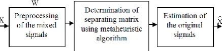
algorithms to solve this problem are FastICA, maximum kurtosis, and maximum likelihood [7-9]. Also, the neural network-based approaches are presented which their separation performances are related to the weights update functions [10]. These functions will be updated according to the distribution of the input signals in order to minimize dependency between the estimated components. The signal distribution in the separation procedure should be estimated and this estimation process reduces the accuracy of the separation procedure. To avoid this problem, metaheuristic-based separation algorithms are presented with no restriction about the signal distribution. An overall block diagram of the separation process is shown in Fig. 1.
In [11], a blind separation method is proposed with this assumption that the source signals are correlated to each other and any additional assumptions do not exist
Fig. 1 Block diagram of a blind separation system.
T
Iranian Journal of Electrical and Electronic Engineering, Vol. 15, No. 3, September 2019 331 about the signal or structures of the mixing matrix. A
pre-separation algorithm is employed based on Wold decomposition principle technique to analyze the predictable segments of the source signals. In [12], the convergence of kurtosis maximization algorithm for separation of the antenna array signals is considered. It is shown that this algorithm is not dependent on the sign of signal kurtosis and can extract the source signals with a proper reconstruction error. In [13], a recursive algorithm is offered to capture the independent components of the input data using the ICA algorithm. Also, the update rules similar to the information maximization algorithm are employed to have a flat convergence in the separation procedure. An ICA-based approach in combination with principal component analysis (PCA) technique is proposed in [14]to separate the acoustic signals in the time-frequency domain. The extracted signals can be separated by comparison of the original acoustic spectrums with the extracted acoustic spectrums.
As mentioned, another way to solve the voice separation problem is based on the meta-heuristic optimization algorithms. In [15-16], a solution for voice separation problem is proposed using maximization of overall kurtosis criterion based on the genetic optimization algorithm. A separation method based on reduction of the mutual information between the mixed signals is introduced in [17] using genetic algorithm (GA) and particle swarm optimization (PSO). Also in [18], the blind separation problem is investigated to yield the estimated signals with lower correlation value. This measure is satisfied based on diagonalization of the correlation matrix for the observed signals using GA. In [19], another method is presented based on the bee colony algorithm to compare the results of blind separation with other optimization methods and different cost functions defined in [16-18]. The structure of this paper is as follows: In Section 2, the blind voice separation problem is explained. In Section 3, the preprocessing procedures of the observed signals are demonstrated. Then, in Section 4, the proposed algorithm based on the empirical mode decomposition and grey wolf optimizer is described. Section 5 includes the implementation details and the performance evaluation of the presented separation algorithm. Finally, the conclusion is expressed in Section 6.
2 Description of Blind Voice Separation Problem
Suppose that Si, i = 1, ..., n are n unknown signals which are as independent as possible. In the linear model of blind separation problem, the source signals are linearly combined with each other by the mixing matrix A as [4]:
.
X A S (1)
where X = [x1, x2, …, xm] includes the mixed signals and
m is the number of the observed signals in the
environment. The separation algorithm proposed in this paper is a linear instantaneous blind voice separation algorithm. This means that the mixing model contains the constant random coefficients. In the noisy environment, this relationship will be as follows:
.
X A S υ (2)
where υ denotes the additive noise signal. The goal in the source separation problem is estimation of the unmixing matrix W without any information about the mixing matrix A. The original source signals are estimated using the captured unmixing matrix based on the following equation [4]:
S Y WX (3)
where Y is estimation of source signals S. It is clear that if W = A-1, the estimated signals involved in Y will be
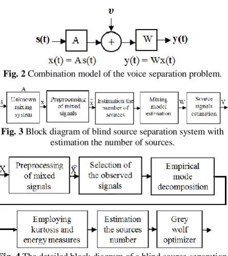
exactly the same as the original sources S. A model for voice separation problem is shown in Fig. 2.
3 Preprocessing Procedures in the Separation Problem
The preprocessing step should be carried out in the first step of the separation procedure to avoid from a complicated optimization algorithm. The preprocessing step contains centering and whitening of the observed signals. Centering is performed using the subtraction of the average values Mi = Ei(xi) from the observed signals to obtain the observed signals with zero mean value. Ei denotes mathematical expectation. At the end of separation algorithm, the calculated mean values are added to the estimated signals. This step leads to the simplified equation in the optimization process. For example, the kurtosis criterion is obtained from the following equation [20]:
2
4 2 2 2
2 2
2 2
4
2 2
3 12
kurtosis( ) 3
4 3 6
Ex E x Ex Ex
x
Ex Ex
ExEx Ex
Ex
(4)
Assuming zero mean for the mixed signals makes it easy to calculate the kurtosis measure using the following equation:
4
2 2
kurtosis x E x 3
E x
(5)
Centering step has an important role in the reduction of computational time. A main part of the proposed cost function involves the kurtosis measure that should be calculated for each population in all iterations of an optimization algorithm. After the centering method,
Iranian Journal of Electrical and Electronic Engineering, Vol. 15, No. 3, September 2019 332 whitening preprocessing is performed. Whitening
converts the mixed signals into the white signals with a linear transmission which their components are uncorrelated to each other and have unit variance. The whitened covariance matrix x, is an identity matrix [21]:
TE x·x I (6)
The principal component analysis (PCA) algorithm is applied to obtain the whitened mixed signals. The eigenvectors in the covariance matrix of the observed signals are utilized:
1 1
1/ 2 2 2
1 1
2 2
1
.
. .
T T
m
diag d d
x FD F x FD F As As D
(7)
where F is the orthogonal matrix of eigenvectors and D is a diagonal matrix of eigenvalues. So, the following equation results:
. T .
.T T . TE x x A E s s A A A I (8)
It is worth mentioning that, using the whitening step, the new mixing matrix will be orthogonal and also the lower number of parameters must be estimated during the optimization process. This means that instead of estimation n2 unknown coefficients of unmixing matrix W, it is enough to capture matrix à with n(n-1)/2 degrees of freedom [20]. Block diagram of the estimation procedure is displayed in Fig. 3.
4 Proposed Separation Algorithm
In this paper, a new separation method is proposed to
Fig. 2 Combination model of the voice separation problem.
Fig. 3 Block diagram of blind source separation system with estimation the number of sources.
Fig. 4 The detailed block diagram of a blind source separation system using an optimization algorithm.
capture blindly voice signals using empirical mode decomposition (EMD) and grey wolf optimizer (GWO). Also, an estimation step is introduced to predict the number of mixed sources in the combination system. Fig. 4 displays the block diagram of the presented algorithm. Each block is explained with details in the following subsections. The proposed separation method is critically-determined that means the number of source and sensors are the same.
4.1 Empirical Mode Decomposition
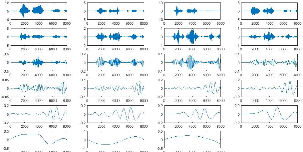
The empirical mode decomposition technique is an adaptive time-space analysis that factorizes an input signal into a finite and often small number of components called intrinsic mode functions (IMF) [22-23]. EMD is based on the Hilbert spectral transform (HT) with a prompt frequency computation and is a suitable processing method for stationary and non-linear signals such as voice signals. This method considers initially oscillatory signals at the level of their local frequencies and sifting process. The constraints in the sifting procedure are: 1) each IMF has the same number of zero-crossings and extreme. 2) each IMF has symmetric envelopes defined by the local extremes. The first IMF usually carries the high-frequency components and can be ignored to remove background random noise signal [22-23]. Fig. 5 shows a speech signal with its IMFs resulted from the EMD technique. The first component is speech signals and other twenty two plots are the captured IMFs from the components with high frequency to the components with low frequency. Also, IMFs obtained from the EMD technique for a mixing signal with four speech components are plots in Fig. 6.
4.2 Estimation of the Source Number
Our proposed scheme to detect the source numbers is detailed as follows. After preprocessing of the observed signals to yield the whitened signals with zero means, five signals with the kurtosis measure value less than the mean of the kurtosis for all ten recorded signals are selected. This number of sources has been experimentally selected. Then, the EMD technique decomposes each selected signals into twenty components according to the time-space analyze. Then, the kurtosis and energy parameters of each obtained IMF for each five selected mixed signals are computed. The number of sources is estimated by two following criterion:
First criterion: Determine the normalized kurtosis value for each IMF of the selected observed signals asKurt i j, ,1 i 20,1 j 5. Kurti j, is the kurtosis value of the i-th IMF component and j-th selected mixed signal. For each mixed signal j, consider the IMF components i with the criterion | Kurti j, Kurt1,j|ε.
1,j
Kurt is related to the first extracted IMF component
for each selected mixed signal. If this condition is
Iranian Journal of Electrical and Electronic Engineering, Vol. 15, No. 3, September 2019 333 Fig. 5 An original speech signal (the first sub-figure in the left of first row) and its IMF components calculated from EMD technique.
Fig. 6 An observed speech signal mixed with four speech signals (the first sub-figure in the left of first row) and its IMF components calculated from the EMD technique.
satisfied, the following condition should be considered. Second criterion: Firstly, the energy parameter for each IMF component of the selected mixed signals is computed. The usual routine in EMD technique is that the energy of signals for the latest extracted components will be less. As mentioned, these components involve low-frequency content with low similarity to the
original voice signal (as shown in Figs. 5 and 6). So, these components should be ignored when the source numbers are calculated. In this criterion, if the normalized energy of each captured IMF obtained from the first condition is lower than the normalized energy of the first IMF, this component is not considered in the counting of the number of sources. Otherwise, the
Iranian Journal of Electrical and Electronic Engineering, Vol. 15, No. 3, September 2019 334 component with a kurtosis and energy parameters that
are close to the parameters values related to the first IMF component (for each selected observed signal), is investigated as one independent source included in each mixed signal.
Performing this routine for these five mixed signals leads to an estimate of the number of original sources that consists of five numbers since an estimated number is obtained after each consideration. Then, the minimum amount of these five estimated numbers is considered as a measure that determines the number of combined sources.
4.3 Grey Wolf Optimization
Grey wolf optimizer (GWO) is a meta-heuristic optimization algorithm inspired by the social hierarchy and lifestyle of grey wolves in nature [24]. Simulation of hunting procedure by considering leadership hierarchy of grey wolves has a prominent role in this optimization process. There are four categories of grey wolves such as alpha, beta, delta, and omega that the first three types (search agents) are employed in the hunting process. This process involves three main steps named searching for prey, prey encircling and attacking step [24]. The hunting technique for different kinds of wolfs in the mentioned steps mathematically models the optimization method for GWO. This algorithm can provide a precise optimization procedure in comparison with other well-known meta-heuristics algorithms [24]. In recent years, this algorithm has been employed to solve optimization problems in the various applications [25-27]. In this paper, this optimization algorithm is employed to obtain the unknown coefficients of the unmixing matrix in the blind source separation problem.
4.3.1 Grey Wolf Optimizer to Solve Voice Separation Problem
In the voice separation problem, it is important to have a quick optimal solution with low complexity. This issue is prominent when the dimension of the optimization problem is high. In this condition, random-based search algorithms outperform the classical methods, since these algorithms work on a comprehensive search space to achieve the appropriate solutions. The GWO algorithm is a population-based meta-heuristic method and as expected has a random-based procedure [28]. This algorithm starts using the suggested responses and tries to make better results for an optimization problem during a series of successive iterations.
The optimization procedure using these algorithms usually involves setting some parameters to improve the solutions and create a new proper population in each iteration. These parameters include the definition of a cost function, the number of unknown problem variables and decision-making parameters. Before the
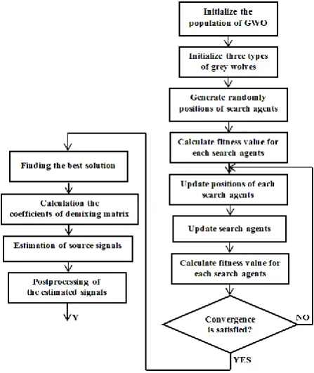
initialization of population, lower and upper bands of each parameter must be specified. When the initial values are determined, the random number generator assigns a value within the permissible limit to all parameters. Various conditions can be considered as stopping criteria in GWO, the predefined number of iterations, a specific cost value or the specified runtime. Block diagram of solving voice separation problem based on GWO is shown in Fig. 7.
4.3.2. The proposed cost function
The basic issue in a cost function designed to solve the blind source separation is maximization of the kurtosis parameter for all estimated signals [16]. This criterion is based on the central limit theorem expressed that the combination of several random variables will have a distribution which its distribution is closer to Gaussian in comparison with each of the primary variables [4, 29].
Therefore, the kurtosis maximization process works in a reverse procedure to yield the separated signals with the kurtosis measure far from the Gaussian variable. In this paper, a new cost function is presented based on the estimation of equiangular tight frames (ETF) to yield an unmixing matrix with independent columns and yield a separation process with more accuracy.
One of the most important steps in the optimization process to solve the voice separation problem is orthogonalization step [30]. It can be concluded that the estimation of demixing matrix coefficients according to the optimization of cost function without orthogonalization step does not lead to the best and
Fig. 7 The overall structure of the proposed blind voice separation method based on GWO.
Iranian Journal of Electrical and Electronic Engineering, Vol. 15, No. 3, September 2019 335 optimal solution. For example, with a cost function
based on the kurtosis criterion, all the estimated signals are identical and involve the source signal with the highest kurtosis value. This solution is the best result obtained using an optimization algorithm since the cost function only involves kurtosis maximization term. In order to prevent this problem, the orthogonalization scheme should be employed. So, before determination of the fitness value for each population in each iteration, the coefficients of the estimated demixing matrix should be orthogonalized. In this paper, I try to achieve the unmixing matrix coefficients with proper orthogonality measure similar to ETF [31]. This problem can be changed as looking for the Gram matrix G = WTW. The
independence measure of an unmixing matrix W is defined as the maximum absolute value of the off-diagonal elements for the Gram matrix G when the columns are normalized. If all off-diagonal elements of G are the same, the dictionary has the minimum coherence or maximum independence [31]. This normalized matrix used to extract the estimated voice signals. ETFs do not exist for any arbitrary matrix dimension. The closest acceptable solution is performed with post-processing of the unmixing matrix. In [32], an iterative projection and rotation (IPR) algorithm is presented to indirectly design Grassmannian frames in two steps. In the first step, the initial Gram matrix is projected into the new one with the structural and spectral constraints. These constraints include thresholding of the off-diagonal coefficients and non-zero eigenvalues of G to ensure ETF characteristics. Next step involves minimization of the residual norm expressed in Y = W.X by a rotating matrix. The cost function according to the mentioned criteria is defined as:
4 2 2
1
1 . 1
2
F [ 3 ( . )
]
n n
i i i j i j
i i j
E Y E Y λ corr y x
λ ETF
W
2| T |
ETF W WW I F
min*
arg
W
W F (9)
where λ1 and λ2 are the weighting coefficients. The
second term of the presented cost function is based on the correlation criterion between the estimated components Y and the observed signals X. The cost function introduced in [18] is based on the correlation reduction between the estimated components with diagonalization of the correlation matrix. But in the proposed cost function, I try to decrease the correlation value between the separated components and the mixing signals.
The last term in this cost function shows Frobenius norm in order to obtain the orthogonal demixing matrix using IPR. The voice signal is a super-Gaussian signal that means the kurtosis of these signals is more than 3.
Also, the absolute value in this cost function causes that the separation process in different circumstances such as in the presence of sub-Gaussian and super-Gaussian signals is performed with high accuracy. In fact, the presented procedure can provide the separation process for multiple super-Gaussian signals, multiple sub-Gaussian signals and also the separation of super-Gaussian and sub-super-Gaussian signals from each other. Therefore, the goal of this optimization procedure is kurtosis maximization of the estimated signals along with the minimization of the correlation criterion between the estimated signals and other observed signals using an orthogonal demixing matrix.
5 Simulation Results
In order to evaluate the performance of the proposed algorithm, different speech signals are selected from TIMIT database for male and female speakers [33]. All input signals are voice sources that are not correlated with each other. This is a main hypothesis to use the central limit theorem in the separation procedure. These signals are combined using mixing matrix A with random coefficients. Performance of the separation procedure using GWO is compared with other mentioned methods using GA [17], PSO algorithm [18], bee colony optimization (BCO) [19], and ICA algorithm [5] in different conditions. The population size of the optimization algorithms is set from 50 to 100 corresponding to the estimated source numbers n. Also, the coefficients of the unmixing matrix W for each optimization algorithm are initialized randomly with n2
parameters. In each iteration, four elite chromosomes are considered. In the GA algorithm, the probability of two points crossover and mutation per each chromosome is Pc = 0.8 and Pm = 0.0025, respectively. The ε parameter defined in Section 4.2 is adjusted to 0.025 according to the experimental results. The stopping criterion is set according to the number of iterations for each estimated source number. All reported results are obtained based on 10 independent runs with the average over all test signals in the mentioned conditions.
MATLAB software was used on a Windows 64-bit based computer with Core i5 3.2 GHz CPU for all experiments.
Different measurements are employed to investigate the performance of the proposed algorithm. One of these measures is the Euclidian distance between the kurtosis vectors of original and estimated signals. In this test, it is assumed that the kurtosis of input voice signals is available:
21
Diff_kurt kurt kurt
n
i i
i
Y S
(10)As expected, the smaller value for this measure gives more similarity between the estimated signals and the
Iranian Journal of Electrical and Electronic Engineering, Vol. 15, No. 3, September 2019 336 original sources. Another measure is the average signal
to noise ratio (SNR) values for all test signals expressed as:
2 2SNR10 logE S E Y S (dB) (11)
It is obvious that the high values of this measure result in the separation procedure with more precision.
5.1 Voice Signals Separation
In this simulation, separation of voice signals with super-Gaussian nature is considered. These signals have been combined together with an unknown mixing matrix. The sampling rate of each signal is 8 KHz. In the first step of the proposed separation procedure, the mixed signals are preprocessed using centering and whitening methods. Then, the IMF components of each recorded signal are obtained using EMD to estimate the number of sources combined in the recorded signals. After setting the source numbers and determining the number of unknown coefficients in the unmixing matrix, GWO is employed to adjust these coefficients according to the defined cost function.
The proposed method is comprised with the separated approaches introduced in [17-19]. As mentioned, in [17] a blind voice separation algorithm was presented using GA with a cost function based on the minimization of the mutual information between the estimated signals. A PSO-based separation algorithm is introduced in [18] based on a cost function included the correlation matrix diagonalization. In [19], a bee colony-based optimization algorithm is presented using a defined cost function based on high order statistics. These methods denote in figures and tables with ((GA-based)), ((PSO-based)) and ((BCO-((PSO-based)) algorithms, respectively. The results of the proposed method are shown with ((GWO-based)).
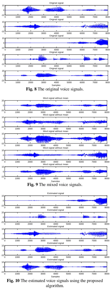
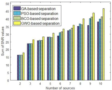
In the first experiment, five voice signals are mixed with each other with an unknown mixing model. The input voice sources S and the mixing signals X are shown in Figs. 8 and 9, respectively. Also, Fig. 10 shows the estimated signals Y resulted from the GWO algorithm in order to separate these five mixing signals. The results of the kurtosis error criterion between the original source signals and demixing signals for separating 2 to 10 sources is shown in Fig. 11. The results of the GWO algorithm in comparison with the presented separation procedure in [17-19] are expressed in this figure. The results of SNR measure for the estimated signals based on (11) for different mentioned methods are reported in Fig. 12. These values are the average results over 10 iterations for each included algorithm. The results show that the estimated signals using the GWO algorithm based on the proposed cost function, which is based on correlation reduction of mixing and demixing signals, and also finding a Grassmannian tight frame to yield independent columns
for the unmixing matrix achieves a more precise estimation than the other separation methods using different optimization process. The differences between the calculated measure values of the proposed procedure and the mentioned algorithms are more prominent when the number of mixing sources increases.
0 1000 2000 3000 4000 5000 6000 7000 8000 -10
0 10
Original signal
0 1000 2000 3000 4000 5000 6000 7000 8000 -10
0 10
Original signal
0 1000 2000 3000 4000 5000 6000 7000 8000 -10
0 10
Original signal
0 1000 2000 3000 4000 5000 6000 7000 8000 -10
0 10
Original signal
0 1000 2000 3000 4000 5000 6000 7000 8000 -20
0 20
Original signal
Samples
Fig. 8 The original voice signals.
0 1000 2000 3000 4000 5000 6000 7000 8000 -20
0 20
Mixd signal without mean
0 1000 2000 3000 4000 5000 6000 7000 8000 -10
0 10
Mixd signal without mean
0 1000 2000 3000 4000 5000 6000 7000 8000 -10
0 10
Mixd signal without mean
0 1000 2000 3000 4000 5000 6000 7000 8000 -10
0 10
Mixd signal without mean
0 1000 2000 3000 4000 5000 6000 7000 8000 -10
0 10
Mixd signal without mean
Samples
Fig. 9 The mixed voice signals.
0 1000 2000 3000 4000 5000 6000 7000 8000 -10
0 10
Estimated signal
0 1000 2000 3000 4000 5000 6000 7000 8000 -20
0 20
Estimated signal
0 1000 2000 3000 4000 5000 6000 7000 8000 -10
0 10
Estimated signal
0 1000 2000 3000 4000 5000 6000 7000 8000 -10
0 10
Estimated signal
0 1000 2000 3000 4000 5000 6000 7000 8000 -10
0 10
Estimated signal
Samples
Fig. 10 The estimated voice signals using the proposed algorithm.
Iranian Journal of Electrical and Electronic Engineering, Vol. 15, No. 3, September 2019 337 Fig. 11 Performance comparison of different methods in terms
of the estimated kurtosis error.
Fig. 12 Performance comparison of different methods in terms of the sum of SNR values.
This result is an important issue in the proposed separation procedure based on the mentioned novelties for improving separation results. It should be noted that the calculated correlation value when the number of sources is low, does not have a noticeable effect on the separation procedure. So, any optimization algorithm which is based on the conventional cost functions will be able to achieve good results. But with increasing the number of sources, employing the correlation measure in the separation procedure of the observed signals will be very effective.
5.2 Separation of Voice Signals in the Presence of White Noise
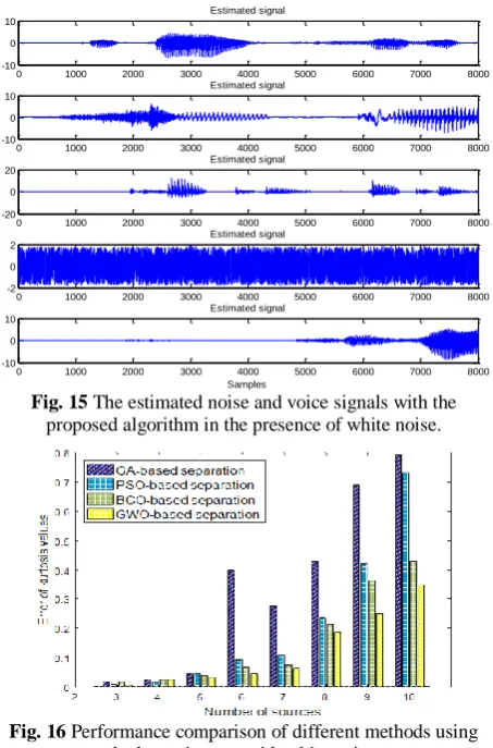
In order to have more evaluation, the performance results of the proposed algorithm are considered in the presence of white noise. This noise signal is selected from Noisex92 database [34]. Fig. 13 shows the source voice signals included white noise. The SNR of noise signal is set to +5dB. The mixed and estimated signals captured using the GWO algorithm in order to separate
these five input signals are displayed in Figs. 14 and 15, respectively. The results of blind voice separation in the presence of white noise with kurtosis error and total SNR measurements values are reported in Figs. 16 and 17, respectively. All the reported values are the result of averaging over 10 iterations for each algorithm. These calculated measure values are precisely consistent with the obtained measure values results that show the proper performance for the proposed method in comparison with other optimization-based separation algorithms. So, the GWO algorithm based on the proposed criterion operates better than other mentioned methods to solve the blind voice separation problem in the presence of white noise. The differences between the obtained results similar to the previous section are more prominent in the separation of more sources that lead to a difficult separation scheme and low accuracy. Another performance evaluation is based on the calculation of computation time for the proposed algorithm. These results reported in Table 1 included the computation time of the separation problem for different optimization-based separation algorithms and ICA-based separation method [5] for different numbers of sources. The reported computation time for the proposed method does not include the first block of separation process involved estimation of the source number. The results show that the proposed algorithm is run a little longer than PSO and BCO. Since the optimization algorithms work based on a random search, the ICA algorithm can be used to separate signals in less time than other methods. However, due to the separation accuracy of the ICA method discussed below, using this method is not particularly suitable when a large number of sources are combined.
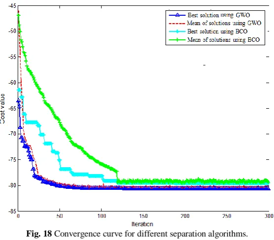
According to the separation results for the investigated criteria, it can be concluded that convergence using GWO occurs faster than the genetic algorithm. It is clear that this distinction in the calculated computation time for the separation process is more prominent when the number of sources is high. The convergence curves of the proposed optimization-based algorithm and BCO-based separation method for demixing five observed signals are shown in Fig. 18. In this figure, the convergence curves of the best solutions and the averages of each solution have been displayed. As can be seen, the solutions average of the GWO algorithm is prominently better than the other mentioned methods. So, it can be concluded that the proposed optimization procedure using the presented cost function in each iteration can pursue precisely the proper population with the best solution. For more consideration about the capability of the proposed method, the average of all results for different algorithms is reported in Table 2. These results are the average value obtained from the separation procedures in the absence and presence of white noise signal. As can be seen from this table, the proposed method that is based on the GWO algorithm and the newly defined cost function achieves
Iranian Journal of Electrical and Electronic Engineering, Vol. 15, No. 3, September 2019 338 significantly better measure values than other
optimization methods to solve the blind voice separation problem. The proposed algorithm obtains the least kurtosis error value and the maximum SNR values in comparison with different considered methods. This superiority is more prominent when the number of mixed sources is high and is consistent with the previous results. Also, the results of ICA algorithm are considerably worse than other optimization algorithms, especially with increasing number of resources.
In the proposed separation method, using a cost function (Eq. (9)) based on correlation and ETF measures leads to a demixing matrix with maximum independence that has a prominent role to obtain the precise results. It should be noted that the computation time of the proposed algorithm increases slightly using this cost function but the separated signals are obtained with minimum overlap to each other. This issue is very important especially when the number of mixed sources is high. So, correlation-based measures in these conditions are fully taken into account in the proposed method.
0 1000 2000 3000 4000 5000 6000 7000 8000 -2
0 2
Original signal
0 1000 2000 3000 4000 5000 6000 7000 8000 -10
0 10
Original signal
0 1000 2000 3000 4000 5000 6000 7000 8000 -10
0 10
Original signal
0 1000 2000 3000 4000 5000 6000 7000 8000 -10
0 10
Original signal
0 1000 2000 3000 4000 5000 6000 7000 8000 -20
0 20
Original signal
Samples
Fig. 13 The original voice signals with white noise.
0 1000 2000 3000 4000 5000 6000 7000 8000 -10
0 10
Mixd signal without mean
0 1000 2000 3000 4000 5000 6000 7000 8000 -10
0 10
Mixd signal without mean
0 1000 2000 3000 4000 5000 6000 7000 8000 -10
0 10
Mixd signal without mean
0 1000 2000 3000 4000 5000 6000 7000 8000 -10
0 10
Mixd signal without mean
0 1000 2000 3000 4000 5000 6000 7000 8000 -20
0 20
Mixd signal without mean
Samples
Fig. 14 The mixing voice signals with white noise.
0 1000 2000 3000 4000 5000 6000 7000 8000 -10
0 10
Estimated signal
0 1000 2000 3000 4000 5000 6000 7000 8000 -10
0 10
Estimated signal
0 1000 2000 3000 4000 5000 6000 7000 8000 -20
0 20
Estimated signal
0 1000 2000 3000 4000 5000 6000 7000 8000 -2
0 2
Estimated signal
0 1000 2000 3000 4000 5000 6000 7000 8000 -10
0 10
Estimated signal
Samples
Fig. 15 The estimated noise and voice signals with the proposed algorithm in the presence of white noise.
Fig. 16 Performance comparison of different methods using the kurtosis error with white noise.
Fig. 17 Performance comparison of different methods using the sum of SNR values in the presence of white noise.
Table 1 Comparison of running time measured in second for different separation methods.
Methods No. of
sources
GWO-based BCO-based [19] PSO-based [18] GA-based [17] ICA [5] 16.58 13.52 12.06 26.1 8 2 27.69 26.41 24.11 73.61 12 3 49.63 48.23 44.62 173.41 27 4 78.28 79.55 77.56 296.68 42 5 131.58 130.64 126.31 534.45 61 6 169.24 168.62 164.74 650.93 85 7 212.35 215.08 210.13 946.78 111 8 245.68 241.31 235.86 1305.8 146 9 304.56 301.22 294.34 1591.7 172 10
Iranian Journal of Electrical and Electronic Engineering, Vol. 15, No. 3, September 2019 339 Fig. 18 Convergence curve for different separation algorithms.
Table 2 Average results of different blind separation methods based on kurtosis error and sum SNR measures.
No.of sources
Methods
ICA [5] GA-based [17] PSO-based [18] BCO-based [19] GWO-based Measure Values
Sum SNR
Kurtosis error
Sum SNR
Kurtosis error
Sum SNR
Kurtosis error
Sum SNR
Kurtosis error
Sum SNR
Kurtosis error
2 18.47 0.001 18.48 0.0014 18.56 0.001 18.48 0.001 19.03 0.001
3 26.63 0.009 26.70 0.018 26.89 0.008 26.53 0.017 27.98 0.008
4 28.15 0.037 29.08 0.035 29.32 0.032 29.16 0.038 30.06 0.023
5 29.81 0.075 31.41 0.063 31.96 0.051 31.35 0.065 32.86 0.039
6 31.02 0.153 34.68 0.118 35.08 0.950 34.72 0.142 36.71 0.079
7 33.15 0.216 36.77 0.173 37.11 0.142 36.65 0.175 38.59 0.088
8 35.72 0.596 41.01 0.326 41.83 0.281 41.20 0.354 43.25 0.223
9 37.61 0.961 44.79 0.507 45.91 0.432 44.87 0.523 46.71 0.308
10 38.29 1.363 44.53 0.872 48.07 0.670 46.38 0.961 49.86 0.431
Table 3 Comparison of the absolute value of OSSR measure for different separation methods. Methods
No.of sources
GWO-based BCO-based [19]
PSO-based [18] GA-based [17]
ICA [5]
0.0263 0.0262
0.0260 0.0261
0.0262 2
0.0378 0.0379
0.0376 0.0384
0.0378 3
0.0434 0.0443
0.0452 0.0461
0.0485 4
0.0531 0.0543
0.0561 0.0572
0.0591 5
0.0608 0.0616
0.0621 0.0632
0.0780 6
0.0722 0.0738
0.0743 0.0758
0.0968 7
0.0843 0.0855
0.0867 0.0877
0.1234 8
0.0903 0.0911
0.0922 0.0943
0.2312 9
0.1007 0.1021
0.1035 0.1061
0.4403 10
To more evaluate the performance of the proposed algorithm, the mean value of the running short-term relative energy measure between original and separated signals is applied. This measure is named with original to separated signal ratio (OSSR) defined as:
2 2
10
1 1 1
1
OSSR log ( ) ( )
T K K
t k k
S t k Y t k
T
(12)where S and Y are the original and separated signals, respectively. Also, T is the total time of signal and K is a square window with 10ms length. If the original and separated signals are exactly similar, this measure has a value close to zero. The larger absolute value of this measure results in a lower similarity between the original and separated signals. In fact, the positive or negative values for this measure indicate dissimilarity. The average OSSR values of each signal for different
Iranian Journal of Electrical and Electronic Engineering, Vol. 15, No. 3, September 2019 340 algorithms are shown in Table 3. It is observed that the
separation efficiency of the proposed algorithm is noticeably better than other mentioned algorithms for different number of mixed sources that are in consistent with the previous results.
6 Conclusion
In this paper, the blind separation problem of voice signals using empirical mode decomposition technique and gray wolf optimization algorithm is considered. The novelty of the proposed method consists of four issues. The first is employing empirical mode decomposition to estimate the number of sources combined in the observed signals. This procedure is based on the energy and kurtosis of the intrinsic mode functions to precisely estimate the source numbers. The second is using iteration projection and rotation algorithm to yield an orthogonal unmixing matrix in order to increase independence between the estimated signals. This problem is more important when the number of sources is high. The third is definition a new cost function based on the correlation reduction between the estimated and the observed signals using diagonalization of the correlation matrix and the last is using grey wolf optimizer algorithm as a population-based meta-heuristic method to achieve unknown coefficients of the unmixing matrix. The results of the proposed algorithm are compared with other optimization-based algorithms such as genetic algorithm, particle swarm optimization, and bee colony algorithm. The performance evaluation of the proposed separation procedure is based on different measures such as kurtosis error criterion between the original and estimated signals and sum of SNR values. The achieved results state that the proposed blind separation scheme is performed more accurately than other mentioned algorithms. These results emphasize the prominent role of the presented cost function that leads to the appropriate performance results especially when the number of sources is high. The experimental results in the presence of white noise emphasize the proper performance of the proposed algorithm.
References
[1] G. D. Pelegrina, L. T. Duarte, and C. Jutten, “Blind source separation and feature extraction in concurrent control charts pattern recognition: Novel analyses and a comparison of different methods,”
Computers & Industrial Engineering, Vol. 92,
pp. 105–114, 2016.
[2] H. Buchner, E. Peterse, M. Eger, and P. Rostalski, “Convolutive blind source separation on surface EMG signals for respiratory diagnostics and medical ventilation control,” in 38th Annual International
Conference of the IEEE Engineering in Medicine
and Biology Society (EMBC), pp. 3626–3629, 2016.
[3] J. Xin and Y. Qi, “Blind source separation and speech enhancement,” in Mathematical Modeling and Signal Processing in Speech and Hearing
Sciences, Springer, Cham, pp. 141–188, 2014.
[4] J. F. Cardoso, “Blind signal separation: statistical principles,” in Proceedings of the IEEE, Vol. 86, pp. 2009–2026, 1998.
[5] S. Choi, H. M. Park, and S
.
Y. Lee, “Blind source separation and independent component analysis: A review”, Neural Information Processing-Letters andReviews, Vol. 6, pp. 1–57, 2013.
[6] G. Lu, M. Xiao, P. Wei, and H. Zhang, “A new method of blind source separation using single-channel ICA based on higher-order statistics,”
Mathematical Problems in Engineering, Vol. 20,
2015.
[7] D. Langlois, S. Chartier, and D. Gosselin, “An introduction to independent component analysis: InfoMax and FastICA algorithms,” Tutorials in
Quantitative Methods for Psychology, Vol. 6,
pp. 31–38, 2010.
[8] J. Ye and T. Huang, “New Fast-ICA algorithms for blind source separation without prewhitening,”
ICAIC 2, pp. 579–585, 2011.
[9] C. Févotte and J. F. Cardoso, “Maximum likelihood approach for blind audio source separation using time-frequency Gaussian source models,” in IEEE Workshop on Applications of Signal Processing to
Audio and Acoustics, pp. 78–81, 2005.
[10]P. S. Huang, M. Kim, M. Hasegawa-Johnson, and P. Smaragdis, “Joint optimization of masks and deep recurrent neural networks for monaural source separation,” IEEE/ACM Transactions on Audio,
Speech, and Language Processing, Vol. 23,
pp. 2136–2147, 2015.
[11]M. R. Aghabozorgi and A. M. Doost-Hoseini, “Blind separation of jointly stationary correlated sources,” IJE Transactions A: Basics, Vol. 16, No. 4, pp. 331–346, 2003.
[12]Z. Ding and T. Nguyen, “Stationary points of a kurtosis maximization algorithm for blind signal separation and antenna beamforming,” IEEE
Transactions on Signal Processing, Vol. 48,
pp. 1587–1596, 2008.
[13]M. T. Akhtar, T. P. Jung, S. Makeig, and G. Cauwenberghs, “Recursive independent component analysis for online blind source separation,” in IEEE International Symposium on
Circuits and Systems, pp. 2813–2816, 2012.
Iranian Journal of Electrical and Electronic Engineering, Vol. 15, No. 3, September 2019 341 [14]A. Sansan, L. Zhen, Z. Nan, and W. Rui, “Blind
source separation based on principal component analysis-independent component analysis for acoustic signal during laser welding process,”
International Conference on Digital Manufacturing
and Automation (ICDMA), Vol. 1, pp. 336–339,
2010.
[15]X. Y. Zeng, Z. Nakao, and G. Yamashita, “Signal separation by independent component analysis based on a genetic algorithm,” in 5th International
Conference on Signal Processing Proceedings,
Vol. 3, pp. 1688–1694, 2000.
[16]D. Mavaddaty and Ebrahimzadeh, “Evaluation of performance of genetic algorithm for speech signals separation,” International Conference on Advances in Computing, Control & Telecommunication
Technologies, pp. 1–4, 2009.
[17]S. Mavaddaty and A. Ebrahimzadeh, “Research of blind signals separation with genetic algorithm and particle swarm optimization based on mutual information,” International Journal of Advanced Developments in Computer Engineering (IJADCE),
Islamic Azad University, Sari Branch, Vol. 1,
pp. 77–88, 2009.
[18]S. Mavaddaty and A. Ebrahimzadeh, “Blind signals separation using genetic algorithm with a novel cost function based on correlation matrix diagonalization and high order statistics,” The 15th National CSI
Computer Conference (CSICC), 2010.
[19]A. Ebrahimzadeh and S. Mavaddati, “A novel technique for blind source separation using bees colony algorithm and efficient cost functions,”
Swarm and Evolutionary Computation, Vol. 14,
pp. 15–20, 2014.
[20]A. Kumar, A. M. Negrat, and A. Almarimi, “A robust watermarking using blind source separation,”
World Academy of Science, Engineering and
Technology, 2008.
[21]J. V. Stone, “Independent component analysis,”
Encyclopedia of statistics in Behavioral Science,
Vol. 2, pp. 907–912, 2005.
[22]M. Lambert, A. Engroff, M. Dyer, and B. Byer,
“Empirical mode decomposition,”
https://www.clear.rice.edu/elec301/Projects02/empir icalMode/process.html.
[23]N. E. Huang, Z. Shen, S. R. Long, M. C. Wu, H. H. Shih, Q. Zheng, N. C. Yen, C. C. Tung, and H. H. Liu, “The empirical mode decomposition and the Hilbert spectrum for nonlinear and non-stationary time series analysis,” Proceedings of the Royal Society of London. Series A: Mathematical,
Physical and Engineering Sciences, Vol. 454, pp.
903–995, 1998.
[24]S. A. Mirjalili, S. M. Mirjalili, and A. Lewis, “Grey Wolf Optimizer,” Advances in Engineering
Software, Vol. 69, pp. 46–61, 2014.
[25]A. R. Tavakolpour-Saleh, S. H. Zare, and H. Badjian, “Multi-objective optimization of Stirling heat engine using gray wolf optimization algorithm,” IJE Transactions C: Aspects, Vol. 30, pp. 895–903, 2017.
[26]E. Sathish, N. Sivakumaran, and S. Sankaranarayanan, “Grey wolf optimization based parameter selection for support vector machines,” International Journal for Computation and Mathematics in Electrical and Electronic
Engineering, Vol. 35, pp. 1513–1523, 2016.
[27]H. Liu, G. Hua, H. Yin, and Y. Xu, “An intelligent grey wolf optimizer algorithm for distributed compressed sensing”, in Computational Intelligence
and Neuroscience, Vol. 6, pp. 1–10, 2018.
[28]R. Storn and K. Price, “Differential evolution: A simple and efficient adaptive scheme for global optimization over continuous spaces,” Journal of Global Optimization, Vol. 23, No. 1, Jan. 1995.
[29]A. Hyvärinen, J. Karhunen, and E. Oja,
Independent component analysis.John Wiley &
Sons, 2001.
[30]T. Tsalaile, S. Sanei, C. Jutten, and J. Chambers, “Sequential blind source extraction for guasi periodic signals with time varying period,” IEEE
Transactions on Biomedical Engineering, 2009.
[31]M. Sustik, J. Tropp, I. Dhillon, and R. Heath, “On the existence of equiangular tight frames,” Linear
Algebra and Its Applications, Vol. 426, pp. 619–
635, 2007.
[32]D. Barchiesi and M. D. Plumbley, “Learning incoherent dictionaries for sparse approximation using iterative projections and rotations,” IEEE
Transactions on Signal Processing, Vol. 61,
pp. 2055–2065, 2013.
[33]W. Fisher, G. Doddington, and K. Goudie-Marshall, “The DARPA speech recognition database: specifications and status,” DARPA
Workshop on Speech Recognition, pp. 93–99, 1986.
[34]A. Varga, H. J. M. Steeneken, M. Tomlinson, and D. Jones, “The Noisex-92 study on the effect of additive noise on automatic speech recognition,” ical
Report, DRA Speech Research Unit, 1992.
Iranian Journal of Electrical and Electronic Engineering, Vol. 15, No. 3, September 2019 342 S. Mavadati was born in Babol, Iran in
1984. He received his B.Sc. degree in Electrical Engineering from University of Mazandaran, Babolsar, Iran, in 2007, the M.Sc. degree in Electrical Engineering from University of Mazandaran, Babolsar, Iran, in 2010, and the Ph.D. degree in Electrical Engineering from Amirkabir University of Technology, Tehran, Iran, in 2016. She is currently an Associate Professor with Electronic Department, Faculty of Technology and Engineering, University of Mazandaran, Babolsar, Iran. Her research interests include speech processing, image processing, artificial intelligence, and optimization algorithms.
© 2019 by the authors. Licensee IUST, Tehran, Iran. This article is an open access article distributed un der the terms and conditions of the Creative Commons Attribution-NonCommercial 4.0 International (CC BY-NC 4.0) license (https://creativecommons.org/licenses/by-nc/4.0/).