A New Bootstrap Based Algorithm for Hotelling’s T2 Multivariate Control Chart

A New Bootstrap Based Algorithm for Hotelling’s T2

Multivariate Control Chart

A. Mostajeran

1

, N. Iranpanah

*1

, and R. Noorossana

2

1_{Department of Statistics, University of Isfahan, 81744, Isfahan, Islamic Republic of Iran} 2_{Department of Industrial Engineering, Iran University of Science and Technology, Tehran, Islamic}

Republic of Iran

Received: 6 September 2015 / Revised: 10 January 2016 / Accepted: 15 February 2016

Abstract

Normality is a common assumption for many quality control charts. One

should expect misleading results once this assumption is violated. In order to

avoid this pitfall, we need to evaluate this assumption prior to the use of control

charts which require normality assumption. However, in certain cases either this

assumption is overlooked or it is hard to check. Robust control charts and

bootstrap control charts are two remedial measures that we could use to overcome

this issue. In this paper, a new bootstrap algorithm is proposed to construct

Hotelling’s T

2

control chart. The performance of proposed chart is evaluated

through a simulation study. Our results are compared to the traditional Hotelling’s

T

2

control chart results and the bootstrap results reported by Phaladiganon

et al.

[13] using in-control and out-of-control average run lengths denoted by ARL0

and

ARL1, respectively. The latter case is obtained when the process mean is subject

to sustained shifts. Numerical results indicate that the proposed algorithm

performs better than the above mentioned methods. The new bootstrap algorithm

is also applied to a real data set.

Keywords: Bootstrap; Hotelling’s T2_{; Multivariate control charts; Average run length; Monte}

Carlo simulation.

*_{Corresponding author: Tel: +983137934593; Fax: +983137934600; Email: [email protected]}

Introduction

One of the major goals of quality control charts is to detect any variation or disturbances in the process as early as possible before many nonconforming products reach the final stage of production. Hence, control charts are widely used in statistical process control activities. In almost all products, quality depends on several quantitative characteristics which need to be controlled or monitored simultaneously. It is well

suggested.

However, a bootstrap method seems to be desirable because it does not require the normality assumption. Bajgier [1] introduced a univariate control chart whose control limits were estimated using a bootstrap method. Seppalaet al. [18] proposed a subgroup bootstrap chart which uses the residuals, i.e. the difference between the mean of a subgroup obtained by bootstrap and each observation in the subgroup. In another study, Liu and Tang [10] suggested a bootstrap control chart that can monitor both independent and dependent observations. Moving block bootstrap was used to monitor the mean of dependent processes. Jones and Woodall [8] compared the performance of bootstrap control charts introduced by Bajgier [1], Seppala et al. [18], and Liu and Tang [10] in non-Normal situations. Polansky [15] used bootstrap method to estimate a discrete distribution, a density estimation method to obtain a continuous distribution, and established control limits. Lio and Park [9] proposed a bootstrap control chart based on Birnbaum-Saunders distribution. Chatterjee and Qiu [3] developed a class of nonparametric cumulative sum (CUSUM) control charts and used bootstrap to find their control limits. Park [12] proposed median control charts whose control limits were established by estimating the variance of the sample median via bootstrap method. Phaladiganon et al. [13] proposed T2 _{multivariate control chart based on}

bootstrap. Noorossana and Ayoubi [11] proposed profile monitoring using nonparametric bootstrap T2 _control

chart. Phaladiganon et al. [14] developed the principal component analysis of control charts for multivariate non-Normal distributions. They used bootstrap method to establish control limits. Psarakis et al. [16] investigated the impact of parameter estimation on the performance of different types of control charts. Faraz

et al. [6] evaluated the in-control performance of the S2

control chart with estimated parameters conditional on the phase I sample.

The use of bootstrap-based T2 _{multivariate control}

chart was first introduced by Phaladiganon et al. [13]. They used bootstrap approach to determine control limits for a T2 _{control chart in which observations did}

not follow a Normal distribution. Although the large sample size is not commonly used for the statistical process control, Phaladiganon et al. [13] applied the large sample size in their approach. While the essence of bootstrap method is based on using resampling from original observations, they resampled usingT2_statistic.

In present paper, a bootstrap approach based on original observations is considered to obtain control limits. The purposed method allows one to use different sample sizes, while the fixed 1000 sample size was

allowed by Phaladiganon’s method. Although the sample size is not essential to be large in the proposed algorithm, but to be able to compare the performances of our algorithm with the Phaladiganon’s algorithm we used the smaller sample sizes. Bootstrap definition ( Efron and Tibshirani [5]) was used to create resample from the original data. Here, ARL1is also calculated for

several defined distributions. Our simulation results are then compared to both traditional Hotelling’s T2 _and

Phaladiganon methods.

In this paper, Hotelling’s T2 _{multivariate control}

charts for monitoring mean of the process have been reviewed. The proposed bootstrap approach for multivariate control charts is then introduced. A simulation study using ARL0 and ARL1 assuming

multivariate Normal, multivariate t, multivariate skew-Normal and multivariate lognormal distributions is then performed. Finally, an application to a real data set is presented.

Multivariate Control Charts for Process Mean

Let a random vector

X

have a p-dimensional Normal distribution, denoted by

N μ

p

( ,

0



₀

)

. It is well known that the statistic

2



(



)

t



(



) ,

T

-1

0 0 0

X

μ

X

μ

can be used to construct a control chart. The

T

2 statistic follows a chi-square distribution withpdegrees of freedom. Hence,

L

_u



χ

2_p,1 is the upper control

limit for the control chart when the vector mean

μ

₀ and covariance matrix



₀are known. This control chart is called a phase II chi-squared control chart. In practice, however,

μ

₀ and



₀ are unknown and should be estimated using sample mean vector

X

and sample covariance matrix S, respectively. The sample mean vector and sample covariance matrix are estimated using the random sample

X

₁

,...,

X

m from

0

( ,

)

p 0



N μ

in phase I. If

X

is a new observation in phase II, we compute

2

(

)

t 1

(

),

T



X X



S



X X



₍₁₎

where

cT

2 has an F distribution with p and m-p

is in control and

μ

₀ and



₀ are known, then average run length of the multivariate control chart is

0 1

ARL 



, where



is the probability of

T

2 exceeding

L

_u. From practical point of view, it is better to use the fundamental definition of ARL0 the average

number of observations required for the control chart to detect a change under the in-control process (Woodall and Montgomery [20]). Furthermore, the out of control ARL (ARL1) of the multivariate chart depends on the

mean vector only through the non-centrality parameter defined as



2

( )

μ

₁



m

δ

t



₀1

δ

,

where

μ

₁



μ

₀



δ

is a specific out of control mean vector. Thus, ARL1is a function of



( )

μ

₁ and

can be calculated using

ARL

₁



1 (1





)

, where



is the probability of an in-control observation while process is indeed out of control.

A New Bootstrap Approach

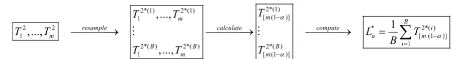
In order to construct a T2_{control limit for the mean} of a process, we have introduced a new algorithm. First, Phaladiganon Bootstrap (PB) algorithm is explained (Figure 1).

1. Compute

T

2 in equation (1) using m in-control observations.

2. Let

T

₁2*( )i

,...,

T

_m2*( )i be a set ofmvalues from the

ith bootstrap sample (i = 1,…,B) randomly drawn from the initial

T

2 statistic with replacement.

3. In each of B bootstrap samples, determine the

(1

)

m





th percentile value given a specified value of



.

4. Determine the control limit by taking the average of

B m

(1





)

th percentile values (

L

*_u



T

_{[ (1 )]m}2*  ).

5. If an observed statistic exceeds

L

*_u, we conclude that process is out of control.

PB algorithm requires a large sample size for calculating the percentiles

T

_{[ (1 )]m}2*( )i , i.e.mmust be large

enough for small



. We assume that

X

₁

,...,

X

_m is a random sample in phase I from unknown distribution and

X

and

S

are the sample mean vector and covariance matrix, respectively.

1. Draw a bootstrap sample

X

* from the observed data

X

₁

,...,

X

_m with replacement.

2. Compute bootstrap statistic

T

2*using

2*

(

*

)

t 1

(

*

).

T



X X



S



X X



₍₂₎

3. Repeat steps 1 and 2, B times to produce

2* 2*

1

,...,

B

T

T

.

4. Determine

B

(1





)

th percentile values

T

2*as the upper control limit

L

*_u



T

_{[ (1 )]}2_B*  .

We use the established control limit to monitor new observations. That is, if the monitoring statistic of the new observations exceeds

L

*_u, we declare those observations as out-of- control signals.

The New Bootstrap (NB) algorithm is applicable for all sample sizes. Therefore, it can be stated that this algorithm is more efficient than the PB algorithm when the sample size is less than 1000. In this algorithm, resampling is done from the main sample not from the observed statistic T2_{. This method requiresB iterations} but the PB algorithm needs to be repeated mB times, thus the new algorithm runs faster than PB algorithm. The proposed algorithm is illustrated in Figure 2.

Figure 1. The Phaladiganon bootstrap algorithm

2*(1) 2*(1) 2*(1)

[ (1 )] 1

2 2 * 2*( )

1 [ (1 )]

1 2*( ) 2*( ) 2*( )

1 [ (1 )]

,...,

1

,...,

,...,

m

m _B

resample calculate compute i

m u m

i

B B B

m m

T

T

T

T

T

L

T

B

T

T

T









  



















Figure 2.A new bootstrap algorithm

2 2 * 2

1

,...,

m



resample



1*

,...,

*B



Compute



T

1*

,...,

T

B*



Calculate



L T

u



[ (1 )]B*

Simulation Study

In this section, a simulation study is performed to evaluate the performance of the proposed algorithm. Notice that there are two considerable ideas in the proposed algorithm.

1. NB algorithm runs faster than PB algorithm. Simulation studies are performed to investigate the performance of our algorithm and compare it to the traditional control chart and PB algorithm.

2. Its efficiency is high even if the sample size is less than 1000.

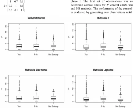
A total ofm=100, 500, and 1000 observations were generated from multivariate Normal (MN), multivariate t (Mt), multivariate skew-Normal (MSN) and multivariate lognormal (MLN) distributions. The distributions MN and Mt are symmetric while MSN and MLN are asymmetric. Each data set contains three variables (p=3). In the simulation, we let µ=[1 1 1]t for MLN distribution and µ=[0 0 0]t _{for other} distributions and the following covariance matrix was considered for MLN distribution:

1 0.7 0.6 0.7 1 0.1 0.6 0.1 1

 

 

   

 

 

This matrix was also used some how for data generating from the other distributions Mt, MSN, and MLN.

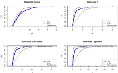
Figures 3 and 4 show the boxplot and cumulative density function (CDF) for T2 _{given in Equation (1)} using exact distribution, simulated data from F distribution withpand m-pdegrees of freedom, andT2* based on NB method for all four distributions. It is not possible to compute distribution of T2 _{by PB method} because it gives only one upper bound. To draw Figures 3 and 4, we generated m=100 observations from each distribution with 1000 Monte Carlo simulation replications.

Figure 4 clearly shows that when distribution is not Normal, the CDF of the NB algorithm is closer to the CDF of T2 _{than F distribution. In other words, the}

proposed NB algorithm provides a more accurate density estimation forT2_.

Comparison of control limits

We generated m =100 in-control observations in phase I. The first set of observations was used to determine control limits for T2_{control charts using PB}

and NB methods. The performance of the control charts is evaluated by generating new observations until theT2

statistic exceeds control limits obtained in phase I. Figure 5 represents T2 _{control charts from the 100}

in-control observations. The false alarm rate was specified

at



= 0.05.

Figure 5 shows that, upper control limits of all three approaches are similar for MN distribution. It also

Figure 4.CDF ofT2_{based on exact distribution, F distribution, and NB algorithm}

shows that all three approaches produce comparable control limits for MN case. When the distribution is not Normal, control limits from traditional T2 _{tend to}

generate higher false alarm rates. The control limits for the traditional Hotelling’sT2_{is not accurate which leeds}

to deviation of rate α = 0.05 from the false alarm. The result for NB and PB algorithms control limits are also close together.

Comparison of in-control with out-control average run length

ARL is the most widely used performance measure for control charts. In this study, we emphasize on the in-control ARL (ARL0), which is defined as the average

number of observations required until an out of control observation is detected under the in-control process.

Furthermore, out of control ARL (ARL1) was

investigated when the process mean vector was contaminated. To calculate ARL1, we changed the mean

of the process using µ = [1 1 1]t _{for MN, Mt, MSN}

distributions, and set µ = [2 2 2]t_{for MLN distribution.}

ARL1 value is calculated as the average number of

observations needed for a control chart to alarm an out of control condition when the process is indeed out of control. Therefore, the corresponding control chart can give better control limits than the other ones, because if ARL1 value is smaller than the deviations of the mean

values of the process, we can be detected sooner. Geometric method is employed to calculate ARL0 and

ARL1 while Phaladiganon et al. [13] have used

binomial method. In the binomial method, first, we generate m data and compute



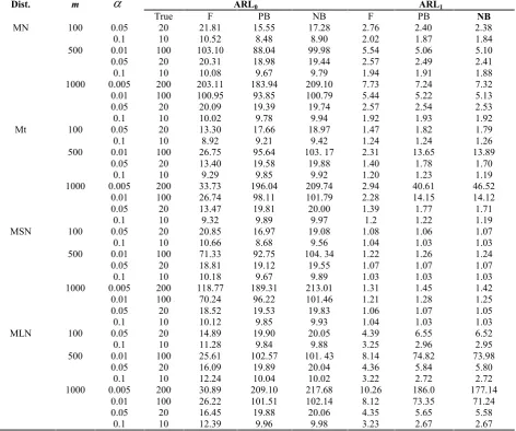
, the percentage of

Table 1.ARL0and ARL1fromT2chart with control limits constructed using F-distribution, PB, and NB algorithms withB=3000

from 20000 simulation runs based on different distributions

corresponding T2 _{that is greater than the upper control}

limit, then calculate

ARL

₀



1



.

The values of ARL0and ARL1were calculated using

20000 simulation runs. When the distribution of the data is MN, the specified ARL0 and the actual ARL0for T2

control chart is expected to be close. Table 1 shows that

for the Normal case, based on ARL0 criterion, the

classical Hotelling’s T2 _{performs better than the other}

two methods but the results show that in all,excepttwo cases, ARL1for the NB algorithm is smaller than F and

PB algorithm. In Table 1, for Mt distribution in comparison with PB algorithm, the performance of the

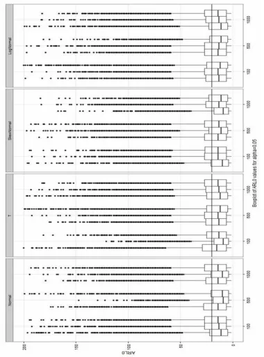
Figure 6.Boxplot of ARL0when simulations are established by F-distribution, PB and NB algorithms

NB method is better for ARL0 criterion except in one

case. Also, ARL1 criterion for NB algorithm is

relatively better than the other methods. Table 1 shows that for the MSN distribution, the traditional Hotelling’s

T2 _{does not perform as expected. In almost all cases,}

ARL1for NB algorithm are less than the ARL1of PB

algorithm. Also for MLN, the NB algorithm performs better than the PB algorithm based on the ARL0

criterion,except forone case. NB algorithm has a better

performance than PB algorithm based on ARL1

criterion.

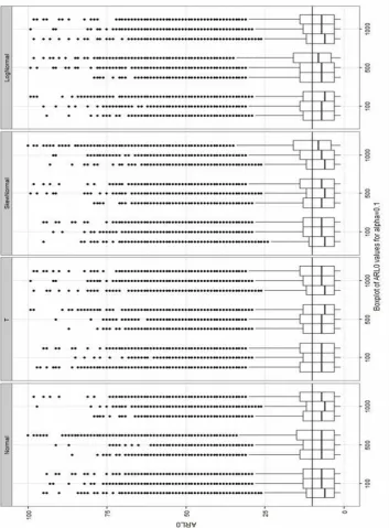
All ARL0values obtained in the simulation study are

shown in Figures 6 and 7 for





0.05

and  0.1,

respectively. Looking at both figures, it can be concluded that, in general, all methods have outlier observations and dispersion of ARL0 values are

different.

Figure 7. Boxplot of ARL0 when simulations are established by F-distribution, PB and NB

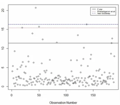
An Application to Real Data

In this section, we consider an example associated with aluminum smelting data. A dataset consisting of 189 observations on 3 variables are collected over time. To assess the multivariate normality of observations, we conducted Royeston’s H test [17]. The p-value of less than 0.001 indicates that this data set does not follow a multivariate Normal distribution (Figure 8). Figure 9 shows the T2 _{control chart whose control limits were}

estimated by F-distribution, PB, and NB algorithms with false alarm rate



= 0.01. The actual ARL0for NB

algorithm is 105 which is similar to the nominal ARL0.

In other words, upper control limit from NB method is more accurate than PB method for calculating ARL0.

Aluminum smelting is an energy intensive, continuous process, and can not easily be stopped and restarted. In view of the possible lack of normality of the data and

considering the enormous cost of process failure, it is worthwhile to monitor process using the NB algorithm.

Results and Discussion

In this paper, we proposed a new bootstrap algorithm in order to obtain the control limits for a control chart which uses observations with unknown distribution because bootstrap method does not require a pre-specified distribution. In comparison to the Phaladiganon’s method, the new bootstrap method proposed in this article is easier to carry out, faster to run, and more accurate in estimation of the density of

T2_{. For non-Normal distributions, the Phaladiganon}

method can be used to determine the limit forT2_control

chart. The Phaladiganon method requires a large sample size, i.e. m =1000, to have a reasonable performance while our new proposed algorithm works well withm< 1000. Furthermore, it is easier to implement. Our simulation results showed that the proposed algorithm is more efficient than the traditional T2_{control chart and}

Phaladiganon method for both Normal and non-Normal cases.

Acknowledgement

The authors are grateful to the graduate office of the University of Isfahan for their support.

References

1. Bajgier S. M. The use of bootstrapping to construct limits on control charts. Proc.Decision Science Institute, San Diego, CA, 1611–1613 (1992). 2. Bersimis S., Psarakis S. and Panaretos J. Multivariate

statistical process control charts:An overview.

Quality & Reliability Engineering International,

23(5): 517–543 (2006).

3.Chatterjee S. and Qiu P. Distribution-free cumulative sum control charts using bootstrap-based control limits. The Annals of Applied Statistics, 3(1): 349-369 (2009).

4. Efron B. Bootstrap methods: another look at the jacknife.The Annals of Statistics,7(1):1–26 (1979). 5. Efron B. and Tibshirani, R. An Introduction to the

Bootstrap. Chapman and Hall. (1993).

6. Faraz A., Woodall W. H. and Cédric H. Guaranteed conditional performance of the S2_{control chart with}

estimated parameters. International Journal of Production Research,53(14): 4405-4413 (2015). 7. Hotelling H., Multivariate quality control. In:

Eisenhart, C., Hastay, M. W., Wills, W. A., eds.

Techniques of Statistical Analysis. New York:

Figure 8. Boxplot of aluminum smelting data

McGraw-Hill, 111–184 (1947).

8. Jones L. A. and Woodall W. H. The performance of bootstrap control charts. Journalof Quality Technology,30: 362–375 (1998).

9. Lio Y. L. and Park C. A bootstrap control chart for Birnbaum–Saunders percentiles.Quality and Reliability Engineering International 24: 585–600 (2008).

10. Liu R. Y. and Tang J. Control charts for dependent and independent measurements based on the bootstrap. Journal of the American Statistical Association,91: 1694–1700 (1996).

11. Noorossanaa R. and Ayoubi M. Profile monitoring using nonparametric bootstrap T2_control chart.Communicationin statistics – Simulation and Computation,41: 302-315(2011).

12. Park H. I. Median control charts based on bootstrap method. Communications inStatistics–Simulation and Computation,38: 558–570 (2009).

13. Phaladiganon P., Kim S. B., Chen V. C., Baek J., and Park S. K. Bootstrap-based

T

2multivariate control charts. Communicationin statistics – Simulation and Computation,40: 645-662 (2011). 14. Phaladiganon P., Kim S. B., Chen V. C., Baek J.,

and Jiang W. Principal component analysis- based control charts for multivariate nonnormal distribution. Expert Systems with Applications, 40: 3044-3054 (2013).

15. Polansky A. M. A general framework for constructing control charts. Quality and Reliability Engineering International,21: 633–653 (2005). 16. Psarakis S., Angeliki K. V., and Philippe C. Some

recent developments on the effects of parameter estimation on control charts.Quality and Reliability Engineering International,30(8): 1113-1129 (2014). 17. Royston J. P. Some techniques for assessing multivariate normality based on theShapiro–Wilk W.Applied Statistics,32(2): 121–133 (1983). 18. Seppala T. Moskowitz H., Plante R. and Tang J.,

Statistical process control via thesubgroup bootstrap.

Journal of Quality Technology,27: 139–153 (1995). 19. Woodall W. H. Controversies and contradictions in

statistical process control.Journal of Quality Technology32(4): 341–350 (2000).