Please cite this article as: N. Torabi, R. Tvakkoli-Moghaddam, E. Najafi, F. Hosseinzadeh-Lotfi, A Two-Stage Green Supply Chain Network with a Carbon Emission Price by a Multi-objective Interior Search Algorithm, International Journal of Engineering (IJE), IJE TRANSACTIONS C: Aspects Vol. 32, No. 6, (June 2019) 828-834
International Journal of Engineering
J o u r n a l H o m e p a g e : w w w . i j e . i rA Two-Stage Green Supply Chain Network with a Carbon Emission Price by a
Multi-objective Interior Search Algorithm
N. Torabia, R. Tavakkoli-Moghaddam*b,c, E. Najafia, F. Hosseinzadeh-Lotfid
a Department of Industrial Engineering, Science and Research Branch, Islamic Azad University, Tehran, Iran b School of Industrial Engineering, South Tehran Branch, Islamic Azad University, Tehran, Iran
c Arts et Métiers ParisTech, LCFC, Metz, France
d Department of Mathematics, Science and Research Branch, Islamic Azad University, Tehran, Iran
P A P E R I N F O
Paper history:
Received 15 January 2019
Received in revised form 15 March 2019 Accepted 21 April 2019
Keywords:
Green Supply Chain Network Multi-objective Optimization Carbon Price
Interior Search Algorithm Meta-Heuristic Algorithm
A B S T R A C T
This paper presented a new two-stage green supply chain network, in which includes two innovations. Firstly, it presents a new multi-objective model for a two-stage green supply chain problem that considers the amount of shortage in the network, reworking, and carbon-trading cost produced in the green supply chain. Secondly, because of the complexity of this model, it uses a new multi-objective interior search algorithm (MOISA) to solve the presented model. The obtained results of the proposed algorithm were compared with the results of other multi-objective meta-heuristics, namely MOPSO, SPEA2, and NSGA-II. The outcomes demonstrate that the proposed MOISA gives better Pareto solutions and indicates the superiority of the proposed algorithm in most cases.
doi: 10.5829/ije.2019.32.06c.05
NOMENCLATURE
Indices Maximum amount of transportation between manufactury warehouse w by vehicle k m and
i Products Maximum amount of transportation between warehouse customer j by vehicle k w and
r Initial parts Maximum amount of transportation between manufactury rework center d by vehicle k m and
n Suppliers Maximum amount of transportation between rework center warehouse w by vehicle k d and
d Rework centers Carbon emissions for producing one unit of product manufactury m i in
m Manufacturer Carbon emissions for reworking on the product d i in rework center
w Warehouses Carbon emissions for transporting one unit of product manufactury m to warehouse w by vehicle k i from
Parameters Carbon emissions for transporting one unit of product i from
warehouse w to customer j by vehicle k
Price of selling and buying carbon emission permit Carbon emissions for transporting one unit of product manufactury m to rework center d by vehicle k i from Demand of product i for customer j Carbon emissions for transporting one unit of product rework center d to warehouse w by vehicle k i from
Maximum limit of supply chain network pollution Factor of converting the fixed cost of establishing manufactury to annual cost m
Fixed cost of establishing manufactory m Factor of converting the fixed cost of establishing warehouse annual cost w to
*Corresponding Author Email: [email protected] (R. Tavakkoli-Moghaddam)
Fixed cost of establishing warehouse w Factor of converting the fixed cost of establishing rework center to annual cost d
Annual cost of selecting supplier n Percent of product i that needs reworking
Fixed cost of establishing rework center d Percent of product reworking i that is turned into sound product after
Production cost of a product unit i in manufactuy m b Current budget for establishing manufactories, warehouses and reworking centers
Cost of purchasing one unit of initial parts n for manufactury m r from supplier Variables
Reworking cost of one unit of product i in rework center d Number of produced products i in manufactury m
Cost of each unit of shortage for product i and customer j Number of reworked product i in rework center d
Transportation cost of one unit of product manufactury m to warehouse w by vehicle k i from Number of initial parts manufactury m r transported from supplier m to
Transportation cost of one unit of product i from warehouse
w to customer j by vehicle k Number of product warehouse w by vehicle i transported from manufactury k m to
Transportation cost of one unit of product manufactury m to rework center d by vehicle k i from Number of product by vehicle k i transported from warehouse w to customer j
center Transportation cost of one unit of product d to warehouse w by vehicle k i from rework center Number of product d by vehicle ki transported from manufactury m to rework
Volume of one unit of product i L ! Number of product warehouse w by vehicle i transported from rework center k d to
Required time to produce product i " Number of shortage for product i for customer j Required time to reworking on the product i E Number of traded carbon emission permit
$ Number of required initial part r to produce product i % Binary decision variable for establishing or not establishing manufactury m
Production capacity (time) of product i in manufactury m % Binary decision variable for establishing or not establishing warehouse w Storage capacity in warehouse w % Binary decision variable for selecting or not selecting supplier n
Supply power of supplier n for initial part r % Binary decision variable for establishing or not establishing rework center d
Reworking capacity(time) on product i in rework center d & Binary decision variable for using or not using the transportation vehicle k between manufactury m and warehouse w
Minimum amount of transportation between manufactury m and warehouse w by vehicle k & Binary decision variable for using or not using the transportation vehicle k between warehouse w and customer j
Minimum amount of transportation between warehouse and customer j by vehicle k w & Binary decision variable for using or not using the transportation vehicle k between manufactury m and rework center d
Minimum amount of transportation between manufactury m and rework center d by vehicle k & Binary decision variable for using or not using the transportation vehicle k between rework center d and warehouse w
Minimum amount of transportation between rework center d and warehouse w by vehicle k
1. INTRODUCTION
Characterized a green supply chain takes a significant role in the supply chain network design. To concern ecological issues, the supply chain management (SCM) forms including item plan, materials determination and sourcing, fabricating, last item conveyance to client and item administration after utilization and time span of usability [1].
In spite of the fact that the ideas of maintainable SCM and green SCM are normally utilized reciprocally all through the supply chain concept, these two ideas are not indistinguishable. Feasible SCM incorporates monetary measurements and ecological and social manageability. Along these lines, maintainable SCM is a more extensive idea in contrast with the green SCM and green SC is a piece of practical supply chain management [2]. Incentives for associations to receive green SCM are distinctive as far as the last client, state offices, private
method, in which some parameters are under uncertainty. Emission trading is one of the economic mechanisms of Kyoto Protocol. In this system, an overall limit on emissions is set for each chain, defined based on permits (also called allowances) to emit up to the level of the overall limit. The chains are allowed to trade these permits. After trading permits, each chain is allowed to emit up to the amount of possessed permits. Hence, each chain should decide on spending costs in order to benefit from environmentally better technology for production, transportation and to minimize emissions or on purchasing permits to meet its own needs. Since trading is performed the open market, the price of emission permits is determined based on supply and demand; which is of high uncertainty.
Fahimnia et al. [4] compared the performance of three meta-heuristic algorithms in solving a complex supply chain.Hassanzadeh et al. [5] proposed new NSGA-II and new MOPSO for a bi-objective supply chain scheduling in a flowshop environment.Chibeles-Martins et al. [6] used the multi-objective meta-heuristic approach for the planning and design of green supply chains, which explores the solution space by using a new local search model. Kumar et al. [7] used self-learning particle swarm optimization for multi-objective models of production and pollution routing problem, in this study time window is assumed. Moresi and Schwartz [8] considered a vertically integrated input monopolist supplying to a differentiated downstream rival. They analyzed vertical delegation as one mechanism for inducing expansion or contraction by the rival/customer. Kumar et al. [9] designed multi objective and multi-period supply chain network with risk and emission, in this study they used NSGA-II for solving problem. Rezaee et al. [10] presented a two-stage model in a stochastic environment to design a green supply chain with carbon price. Qu et al. [11] proposed the taking inventory control out of the hands of competitive or exclusive retailers and assigning it to a manufacturer increases the value of a supply chain especially for goods whose demand is highly volatile. Kadzinski et al. [12] evaluated the applicability of different multi-objective optimization strategies for solving green supply chain problems. Fakhrzad et al. [13] developed a new multi product, multi period, and multi level closed-loop green supply chain planing model under uncertain conditions.
This paper contains two basic innovations. Firstly, a new supply chain model is applied in two stages, with multi-objective functions and the number of shortages and reworks in the model, in which this supply chain model has not been presented in this form of modeling so far in any previous research. Secondly, this new MOISA has not been applied to the supply chain so far, and this algorithm yields very good results in this study. In section 2 of this paper materials and methods presented. In section 3, results and discussion are provided, and a
numerical example is used to demonstrate the adequacy of the model and proposed algorithm. In section 4, conclusion and further studies are provided. In section 5, references are presented.
2. MATERIALS AND METHODS
The model of the intended problem included a multi-objective and two-stage mathematical model. The innovation of this research is to consider the multi-objective and trade off among these multi-objectives in supply chain network and to consider reworking in this multi objective model. Another innovation in this research is the application of an MOISA algorithm for solving a multi-objective supply chain model, which has not been used for these types of two-stage models yet.
2. 1. Two-Stage Green Supply Chain Network
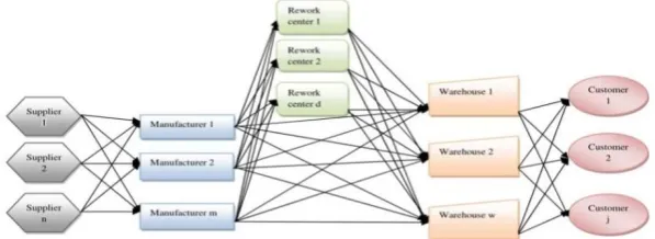
The model presented in this study consists of two stages. Its first stage includes the selection of supplier, selection and location of establishing manufacturer, reworking centers, and warehouses. These places were selected with certain capacities among potential places. The second stage included the determining amount of products, transportation, type of selected vehicle for moving the products, the amount of initial materials purchased from each supplier, the amount of products that need reworking, the amount of created shortage for the final customer demand and the amount of carbon emission permit. The final products in this model are only delivered to customers through warehouses, so that the products are sent from manufacturer to warehouses or from manufacturer to reworking centers and then from reworking centers to warehouses. Finally, the products are delivered to the customers from warehouses. There are minimum and maximum amounts of transportation in the model and the transportation amount that should be certainly in this range. Figure 1 shows the schematic view of the desired model. After that, parameters, variables and model are presented.
Figure 1.Schematic view of a green supply chain
capacity of rework centers meet the number of parts which need reworking. Equation (12) guarantees that the capacity of suppliers is more than the number of required initial parts. Equation (13) shows the type of decision variables for the model’s first phase. The objective function (14) is related to carbon production costs. Equation (15) guarantees the more capacity(time) of manufactories than the required time to produce products. Equation (16) states the relationship between the number of parts, which need reworking and the number of parts which enter rework centers. Equation (17) guarantees the more capacity(time) of reworking center than the Required time for reworking. Equation (18) indicates the number of required parts for producing the final products. Equation (19) indicates the more capacity of suppliers than the number of required initial parts for production. Equation (20) indicates the relationship between the number of sound products and the number of sound products sent from manufactories to warehouses. Equation (21) shows the relationship between the numbers of products which need reworking and the number of products sent from manufactories to rework centers. Equation (22) shows the relationship between the number of sound products after reworking and the number of products sent from rework centers to warehouses. Equation (23) guarantees that the capacity of warehouses is more than the number of products sent from manufactories and rework centers to warehouses. Equation (24) shows the equality between the products imported to warehouse and the products exported. Equation (25) shows the relationship between the number of products imported to warehouse and the amount of shortage than the customer demand. Equation (26) shows the number of carbon emission permit than production pollution and transportation pollution. Equations (27) to (30) show the minimum and maximum limitations for transportation. Equations (31) to (33) show the type of decision variables for the model’s second phase.
Min ∑ lt- -f-F- (1)
Min ∑ lt f F (2)
Min ∑ f0 0F0 (3)
Min ∑ lt f F (4)
Min Q2F, F , F , F 4 (5)
∑ f- -F-+ ∑ f F + ∑ f F ≤ b (6)
∑ F- -≥ 1 (7)
∑ F ≥ 1 (8)
∑ F ≥ 1 (9)
21 − β 4 ∑ ∑ c- -F-+ β ∑ ∑ c F ≥ ∑ ∑ d> > (10)
β ∑ ∑ c- -F-≤ ∑ ∑ c F (11)
∑ c0 ?0F0 ≥ ∑ ∑ d> >α? ∀r (12)
F- , F , F0, F ϵ {0,1} (13)
Q2F, F , F , F 4 = Min ∑ ∑ ∑ ∑ ct- ! - !L- !
+ ∑ ∑ ∑ ∑ ct> ! >!L >!
+ ∑ ∑ ∑ ∑ ct- ! - !L- !
+ ∑ ∑ ∑ ∑ ct! !L !+ ∑ ∑ cm- -Q-
+ ∑ ∑ cd QD
+ ∑ ∑ ∑ cs? - 0 ?0-R?0-+ ∑ ∑ cb> >B > + πE
(14)
∑ μ Q-≤ ∑ c-F- ∀m (15)
∑ QD = ∑ β Q- - ∀i (16)
∑ μ QD ≤ ∑ c F ∀d (17)
∑ R0 ?-0= ∑ α?Q- ∀r, m (18)
∑ R- ?-0≤c?0F0 ∀r, n (19)
∑ ∑ L- ! - != QD ∀i, d (21)
∑ ∑ L! != β QD ∀i, d (22)
∑ ∑ ∑ μ L- ! - !+ ∑ ∑ ∑ μ L! !≤ c F ∀w (23)
∑ ∑ L> ! >!= ∑ ∑ L- ! - !+ ∑ ∑ L! ! ∀i, w (24)
∑ ∑ L! >!+ B >= d> ∀i, j (25)
∑ ∑ ∑ ∑ et- ! - !L- !+
∑ ∑ ∑ ∑ et> ! >!L >!+ ∑ ∑ ∑ ∑ et- ! - !L- !+
∑ ∑ ∑ ∑ et! !L !+ ∑ ∑ em- -Q-+
∑ ∑ ed QD − cap = E
(26)
lb- !G- !≤ ∑ μ L- !≤ ub- !G- ! ∀m, w, k (27)
lb >!G >! ≤ ∑ μ L >!≤ ub >!G >! ∀w, j, k (28)
lb- !G- !≤ ∑ μ L- !≤ ub- !G- ! ∀m, d, k (29)
lb !G !≤ ∑ μ L !≤ b !G ! ∀d, w, k (30)
F- , F , F0, F , G- ! , G >! , G- !, G ! ϵ {0,1}
∀m, w, n, d, k, j (31)
Q- , QD , B > , R?0- , L- ! , L >! , L- !, L !≥
0 and integer ∀i, m, w, n, d, k, j (32)
E is free (33)
2. 2. Multi-objective Interior Search Algorithm
In the multi-objective interior search algorithm (MOISA), concepts of the ISA [14] are used in conjunction with the principles of the crowding distance and non-dominated sorting. In the proposed algorithm, those stages of process that require sorting out the original population use the two mentioned principles for this purpose. By considering literature [15] meta-heuristic multi objective interior search algorithm used for solving gscm model presented in this paper. The pseudo code of MOISA is as follows:
Initialization
while any stop criteria is not satisfied use the non dominated sorting use the crowding distance find the Pareto fronts
choose one of the solution in the first Pareto front as xjgb
for i=1 to n
if xgb
xjgb = xj-1gb +rn × λ
else if r1 ≤α
xjm,i = r3 xj-1i +(1-r3) xjgb
xji= 2 xjm,I - xj-1i
else
xji=LBj +(UBi -LBj )×r2
end if
check the boundaries except for decomposition elements end for
for i=1 to n
evaluate the f(xij)
xij =XY Z [Y \ ] Z^ [Y
_`\
Y _` a
end for
end while
3. RESULTS AND DISCUSSION
Numerical examples should be used to guarantee the efficiency of the presented model. Four meta-heuristic algorithms, namely MOPSO, NSGA-II, SPEA 2 and MOISA, are used to solve the given examples. The following four comparative factors are considered to determine the algorithms that have a better performance in solving the proposed model.
1. Mean ideal distance (MID): This criterion calculates the mean Pareto solutions from the coordinate’s origin. The less is this criterion, the more is the algorithm efficiency.
2. Spacing (S): This criterion calculates the relative distance of consecutive solutions. The less is the index, the better it is [16].
3. Number of Pareto solutions (NOS): The more is the number of Pareto solutions, the more optimal will be that method.
4. Solving time (TIME): This factor is measured based on the number of function evaluations, the less is the better.
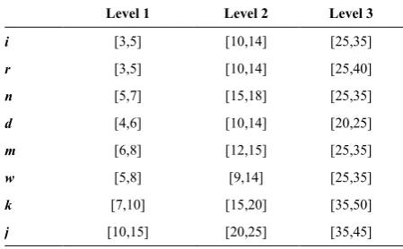
Numerical examples are considered at three levels of small, medium and large. The values of the model’s indices for these three levels are given in Table 1. Table 2 shows the parameter setting results from Taguchi method. The stopping condition of algorithms is equal to the number of function evaluation=10000. Each example is run 50 times with each algorithm. Table 3 shows the average results of model solving.
TABLE 1. Values for three levels of the indices.
Level 3 Level 2
Level 1
[25,35] [10,14]
[3,5]
i
[25,40] [10,14]
[3,5]
r
[25,35] [15,18]
[5,7]
n
[20,25] [10,14]
[4,6]
d
[25,35] [12,15]
[6,8]
m
[25,35] [9,14]
[5,8]
w
[35,50] [15,20]
[7,10]
k
[35,45] [20,25]
[10,15]
TABLE 2. Parameter setting results from Taguchi method
NSGA II MOPSO SPEA II MOISA
Population size= 1000 Mutation Rate=
0.1 P Crossover=0.7
P Mutation=0.2
Population size= 1000 Repository
Size=300 Inertia Weight=0.5
Personal Learning Coefficient=1 Global Learning
Coefficient=2 Number of Grids
per Dimension=10
Alpha=0.1 Beta=2 Gamma=2
Mutation Rate=0.1
Population size= 1000 Archive Size=500 P Crossover=0.7
P Mutation=0.3
Population size= 1000 Alpha=0.4
TABLE 3. Average results of model solving
Criterion
Level 1 Time NOS S MID
NSGAII 920.797 40 3.3438×10^5 2.2132×10^7 SPEA-2 850.15 43 3.0012×10^5 2.0744×10^7 MOPSO 950.51 39 3.4431×10^5 2.3332×10^7 MOISA 880.31 48 2.8911×10^5 2.0232×10^7
Level 2 Time NOS S MID
NSGAII 16854.23 41 7.8823×10^6 1.8061×10^9 SPEA-2 15120.16 47 7.2451×10^6 1.7319×10^9 MOPSO 17001.65 38 8.2141×10^6 2.0198×10^9 MOISA 14790.21 46 6.9917×10^6 1.6531×10^9
Level 3 Time NOS S MID
NSGAII 294671.34 40 1.2556×10^7 8.4346×10^9 SPEA-2 290154.23 43 1.1144×10^7 8.1978×10^9 MOPSO 295771.98 35 1.5071×10^7 8.7712×10^9 MOISA 288156.32 47 1.0142×10^7 8.0011×10^9
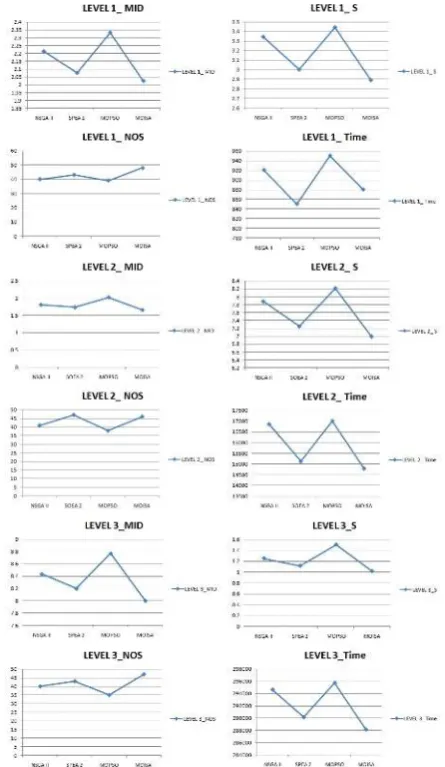
Figure 2 shows the average results obtained by solving the model using different algorithms. In the first level, the performance of the proposed MOISA is better in the MID, S and NOS criteria. The performance of the SPEA-2 algorithm is better in criterion TIME. In the second level, the performance of the proposed MOISA is better in the MID and S criteria. The performance of the SPEA-II algorithm is better in criterion NOS. The performance of MOISA algorithm was better in criterion TIME. In the third level, the performance of the proposed MOISA is better in MID, S, NOS and TIME criteria.
Figure 2. Values of the criteria for the average results
4. CONCLUISION
in the field of fuzzy, interval and gray numbers. Additionally, by combining single-objective meta-heuristic algorithms, we can also create new methods for solving multi-objective models by combining their properties together. Furthermore, other factors (e.g., considering products return by customers, initial inventory, and time periods for production) can be considered in the model.
5. REFERENCES
1. Srivastava, S.K., “Green supply-chain management: A state-of-the-art literature review”, International Journal of
Management Reviews, Vol. 9, No. 1, (2007), 53–80.
2. Zanjirani Farahani, R., Asgari, N., and Davarzani, H., Supply Chain and Logistics in National, International and Governmental Environment - Concepts and Models, Springer-Verlag Berlin Heidelberg, (2009).
3. Zhu, Q., and Sarkis, J., “An inter-sectoral comparison of green supply chain management in China: Drivers and practices”,
Journal of Cleaner Production, Vol. 14, No. 5, (2006), 472–
486.
4. Fahimnia, B., Davarzani, H., and Eshragh, A., “Planning of complex supply chains: A performance comparison of three meta-heuristic algorithms”, Computers & Operations
Research, Vol. 89, (2018), 241–252.
5. Hassanzadeh, A., Rasti-Barzoki, M., and Khosroshahi, H., “Two new meta-heuristics for a bi-objective supply chain scheduling problem in flow-shop environment”, Applied Soft
Computing, Vol. 49, (2016), 335–351.
6. Chibeles-Martins, N., Pinato-Varela, T., Barbosa-Povoa, A., and Novais, A.Q., “A multi-objective meta-heuristic approach for the design and planning of green supply chains - MBSA”,
Expert Systems with Applications, Vol. 47, (2016), 71–84.
7. Kumar, R.S., Kondapaneni, K., Dixit, V., Goswami, A., Thakur, L.S., and Tiwari, M.K., “Multi-objective modeling of production and pollution routing problem with time window: A
self-learning particle swarm optimization approach”,
Computers & Industrial Engineering, Vol. 99, (2016), 29–40.
8. Moresi, S., and Schwartz, M., “Strategic incentives when supplying to rivals with an application to vertical firm structure”, International Journal of Industrial Organization, Vol. 51, (2017), 137–161.
9. Kumar, R.S., Choudhary, A., Babu, S.I., Kumar, S.K., Goswami, A., and Tiwari, M.K., “Designing multi-period supply chain network considering risk and emission: a multi-objective approach”, Annals of Operations Research, Vol. 250, No. 2, (2017), 427–461.
10. Rezaee, A., Dehghanian, F., Fahimnia, B., and Benita, B., “Green supply chain network design with stochastic demand and carbon price”, Annals of Operations Research, Vol. 250, No. 2, (2017), 463–485.
11. Qu, Z., Raff, H., and Schmitt, N., “Incentives through inventory control in supply chains”, International Journal of Industrial
Organization, Vol. 59, (2018), 486–513.
12. Kadziński, M., Tervonen, T., Tomczyk, M., and Dekker, R., “Evaluation of multi-objective optimization approaches for solving green supply chain design problems”, Omega, Vol. 68, (2017), 168–184.
13. Fakhrzad, M.B., Talebzadeh, P., and Goodarzian, F., “Mathematical Formulation and Solving of Green Closed-loop Supply Chain Planning Problem with Production, Distribution and Transportation Reliability”, International Journal of
Engineering - Transactions C: Aspects, Vol. 31, No. 12,
(2018), 2059–2067.
14. Gandomi, A. H., “Interior search algorithm (ISA): A novel approach for global optimization”, ISA Transactions, Vol. 53, No. 4, (2014), 1168–1183.
15. Torabi, N., Tvakkoli-Moghaddam, R., Najafi, E., and Hosseinzadeh-Lotfi, F., “Multi-objective interior search algorithm for optimization: A new multi-objective meta-heuristic algorithm”, Journal of Intelligent & Fuzzy Systems, Vol. 35, No. 3, (2018), 3307–3319.
16. Schott, J., “Fault Tolerant Design Using Single and Multicriteria Genetic Algorithm Optimization,” Master’s thesis, Massachusetts Institute of Technology, (1995).
A Two-Stage Green Supply Chain Network with a Carbon Emission Price by a
Multi-objective Interior Search Algorithm
N. Torabia, R. Tavakkoli-Moghaddamb,c, E. Najafia, F. Hosseinzadeh-Lotfid
a Department of Industrial Engineering, Science and Research Branch, Islamic Azad University, Tehran, Iran b School of Industrial Engineering, South Tehran Branch, Islamic Azad University, Tehran, Iran
c Arts et Métiers ParisTech, LCFC, Metz, France
d Department of Mathematics, Science and Research Branch, Islamic Azad University, Tehran, Iran
P A P E R I N F O
Paper history:
Received 15 January 2019
Received in revised form 15 March 2019 Accepted 21 April 2019
Keywords:
Green Supply Chain Network Multi-objective Optimization Carbon Price
Interior Search Algorithm Meta-Heuristic Algorithm ! " # . .%! & ' ( )
%*+ , - ./ 0 1
! 2*
" 34 5 4 1
4 . - -4 " 6 ! 7 8 . 9
"9 : # ' 1 1
" ; <*0 =< > ./ , ) MOISA ( 5& ' A<! %! B.C # =< > & %! D < .
> =< > < , 1 , - ./
'E MOPSO ، SPEA2 NSGA-II * 9 " 5 C D < .%!
4 -=< > B.C # F 0 # <B 3 <C 1
B.C # =< > *
>
=< > %! 3 'G <B D < -.