Improved confidence interval estimation of the population standard deviation using ranked set sampling: A simulation study

http://jbe.tums.ac.ir

Please cite this article in press as: AlbatinehAN, Wilcox ML, Zogheib B, Kibria GBM. Improved confidence interval estimation of thepopulation standard deviation using ranked set sampling: A simulation study. J Biostat Epidemiol. 2018; 4(3): 173-183

Original Article

Improved confidence interval estimation of the population standard deviation using ranked set sampling: A simulation study

Ahmed N. Albatineh1_{*, Meredith L. Wilcox}2_{, Bashar Zogheib}3_{, Golam B.M. Kibria}4

1 _{Department of Community Medicine and Behavioral Sciences, Faculty of Medicine, Kuwait University, Kuwait} 2 _{Department of Epidemiology, Stempel College of Public Health, Florida International University, Miami, USA} 3 _{Department of Natural Sciences, Faculty of Science, American University of Kuwait Kuwait}

4 _{Department of Statistics, College of Science, Florida International University Miami, Florida, USA}

ARTICLE INFO ABSTRACT

Received: 22.01.2017 Revised 12.02.2018 Accepted 16.03.2018

Background & Aim: The sample standard deviation S is the common point estimator of σ, but S is sensitive to the presence of outliers and may not be an efficient estimator of σ in skewed and leptokurtic distributions. Although S has good efficiency in platykurtic and moderately leptokurtic distributions, its classical inferential methods may perform poorly in non-normal distributions. The classical confidence interval for σ relies on the assumption of normality of the distribution. In this paper, a performance comparison of six confidence interval estimates of σ is performed under ten distributions that vary in skewness and kurtosis.

Methods and Material: A Monte Carlo simulation study is conducted under the following distributions: normal, two contaminated normal, t, Gamma, Uniform, Beta, Laplace, exponential and χ2 with specific parameters. Confidence interval estimates obtained using the more powerful ranked set sampling (RSS) are compared with the traditional simple random sampling (SRS) technique. Performance of the confidence intervals is assessed based on width and coverage probabilities. A real data example representing birth weight of 189 newborns is used for assessment.

Results: It is not surprising that for normal data most of the intervals were close tot he nominal value especially using RSS. Simulation results indicated generally better performance of RSS in terms of coverage probability and smaller interval width as sample size increases, especially for contaminated and heavy-tailed skewed distributions.

Conclusion: Simulation results revealed that the use of RSS improved greatly the coverage probability. Also, it was found that the interval labeled (III) due to Bonett (2006) had the best performance in terms of coverage probability over the wide range of distributions investigated in this paper and would be recommended for use by practitioners. There may be a need to develop nonparametric intervals that is robust against outliers and heavy-tailed distributions.

Key words:

Interval estimation; Standard deviation; Ranked set sample; Coverage probability; Simulations

Introduction

Confidence interval estimation plays an important part in statistical inference about a population parameter and evaluating the accuracy of its estimator. A confidence interval for a parameter represents a set of plausible values for that parameter along with a confidence level. For example, if σ is the standard deviation of a population, then we seek

two endpoints L, U such that P(L≤σ≤U) =1-α for a given level α. The sample standard deviation S is the common point estimator of σ, but S is very sensitive to the presence of outliers in the data and may not be an efficient estimator of σ in skewed and leptokurtic distributions. Although S has good efficiency in platykurtic and moderately leptokurtic distributions, its classical inferential methods may perform poorly in non normal distributions, see Abou-Shawiesh et al. (1) for a discussion. The classical confidence interval for σ relies on the assumption of normality of the distribution. This interval is highly sensitive to the presence of outliers and/or

_____________________________________________________

* Corresponding Author: Ahmed N. Albatineh

Department of Community Medicine and Behavioral Sciences P.O Box 24923, Safat 13110, Kuwait

departure from normality as demonstrated by Lehman and Romano (2). As a result, many researchers attempted to develop an alternative to the classical interval estimate of σ. The key question is which of those available intervals work best and under which setting? Hence there is a need for a comprehensive comparison between such interval estimates of σ.

Abou-Shawiesh et al. (1) performed a simulation study comparing seven confidence intervals for σ using data from normal, χ2_{, and}

Log-Normal distributions. Kittani and Zghoul (10) introduced two confidence intervals for σ based on the asymptotic distribution of the average absolute deviation from the median (AMAD) and mean absolute deviation (MAD) and compared their performance with the classical χ2 _{interval over a range of distributions.}

Hummel et al. (9) compared the performance of four interval estimates of σ for a range of sample sizes and data generated from a number of distributions. Bonnett (5) proposed an approximate confidence interval for σ and showed that it was near exact under normality with excellent small sample properties under non normality and compared its performance with the classical χ2 _{interval. Cojbasic and Tomovic}

(7) compared the performance of four methods for estimating confidence interval for the variance of only the exponential distribution aiming to remove most of its skewness. Citing the importance of estimating the kurtosis and its impact on the performance of the interval estimate, Burch (6) considered a number of kurtosis estimators combined with large sample theory to construct approximate confidence intervals for σ and compared performance of four interval estimates for σ over a range of distributions.

While these studies introduced new methods for estimating σ, there is a need for a more comprehensive simulation study comparing many intervals under a wide range of distributions. For that reason, six interval estimates of σ were chosen from these studies and will be compared using data generated from ten distributions in the current study, making it a more comprehensive one. Moreover, the more powerful ranked set sampling (RSS) technique will be implemented and compared with the classical simple random sampling (SRS) technique which makes this study unique in this regard. The more powerful RSS can be used to

obtain estimates of μ and σ in situations where the variable of interest is too expensive or can't be easily measured, but can be easily ranked. McIntyre (12) was the first to suggest using RSS to estimate population mean instead of SRS and the idea was later developed by Takahasi and Wakimoto (18) using mathematical theory to support their claim. Stokes (17) proposed an estimator for the variance of a ranked set sample data and showed that the estimator is asymptotically unbiased and asymptotically more efficient than the sample variance of a simple random sample of the same number of observations regardless of presence of errors in ranking. MacEachern et al. (11) proposed an alternative estimator for the variance which is unbiased and more efficient than Stokes's estimator even when the underlying distribution is not normal and the ranking of the elements is not perfect. MacEachern et al. (11) estimator of σ2 _{performs well for small to moderate sample}

sizes and is asymptotically equivalent to Stokes (17) estimator.

In this paper, performance comparison of six confidence intervals for estimating the population σ using RSS compared with the usual SRS technique using data from ten distributions with varying skewness and kurtosis. The estimator of the variance of a ranked set sample proposed by MacEachern et al. (11) will be used in the simulations. The comparison will be based on coverage probability and intervals width which seems to be the major factors for comparison, see Albatineh et al. (3) and Terpstra and Wang (19) for a discussion.

Methods

Unbiased estimate of μ and σ using ranked set sample

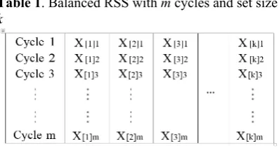
Suppose that we are interested in obtaining an RSS of size n from a population. First, a SRS of size k observations are selected and rank ordered on an attribute of interest. The observation that is determined to be the smallest is the first element of the RSS and is denoted X[1]1 and the

remaining k-1 units are discarded. A second SRS of size k is selected from the population and ranked the same way and the second smallest observation is selected and denoted X[2]1. In a

similar fashion, X[3]1, X[4]1,...,X[k]1 are selected,

hence X[1]1, X[2]1,...,X[k]1 represent our first

http://jbe.tums.ac.ir

175

independent cycles yielding the balanced RSS of size n shown in Table 1.

The complete balanced RSS with set size k

and m cycles is given by {X[r]i: r=1, 2,...,k;

i=1,2,...,m}. The term X[r]i is called the r-th

judgment order statistic from the i-th cycle. It is the observation that is judged to be the r-th order statistic from one of the k sets in the i-th cycle, see MacEachern et al. (11) for discussion. Assume that the underlying distribution has finite mean μ and variance σ2_{, Stokes (17)}

proposed an estimator of σ2 _{based on RSS given}

by

2 2

[ ] [ ]

1 1 1 1

1 1

ˆ ( ˆ) , where ˆ

1

m k m k

r i r i

i r i r

X X

km km

σ μ μ

= = = =

= − =

−





(1)

Stokes (17) showed that this estimator is a biased estimator of σ2_{, but it is asymptotically}

unbiased as either k or m approach ∞. Moreover, Stokes (17) indicated that the RSS estimator

μ

ˆ

has more precision over the sample mean; say

y

obtained using SRS because of independence of the order statistics composing the ranked set sample. In fact, the author showed that var (

y

) ≥ var (

μ

ˆ

). The balanced RSS is used in this paper. The estimator of the variance of a RSS proposed by MacEachern et al. (11) will be implemented in the simulations since it has been shown to perform very well for small as well as large ranked set samples, which is an improvement on Stokes estimator (17). This estimator is given by

(

)

2 1

ˆ (k 1)MST (mk k 1)MSE km

σ = − + − +

(2)

where MST (Mean Square Treatment) and MSE (Mean Square Error) are obtained from an analysis of variance performed on the ranked set sample data with the judgment class used as the factor and are given by

2 2

[ ] [ ] [ ].

1 1 1 1

1 _ˆ 1

( ) ( )

1 1

m k m k

r i r i r

i r i r

MST X X X

k = = μ k = =

= − − −

−



−



(3)

2

[ ] [ ]. [ ]. [ ]

1 1 1

1 1

( ) , where

( 1)

k m m

r i r r r i

r i i

MSE X X X X

k m = = m =

= − =

−





(4)

Confidence intervals for σ

In this section, six widely used confidence intervals for estimating σ are presented.

Exact confidence interval (I)

Let

x x x

1

, , , ,

2 3 

x

n_{be an independent and}

identically distributed random sample from a normal distribution with finite mean μ and variance σ2_{, i.e. X~N (μ, σ}2_{), then}

2

2 2

2 2

1

( 1) 1

( ) ( 1)

n

i i

n S

x x _χ n

σ σ =

− ₌



_{−  −}

(5)

Therefore,

2

2 2 2 2 2

2

( ) (1 ) ( ) (1 )

2 2 2 2

( 1)

( ) ( n S )

P χ _α χ χ _α P χ _α χ _α

σ − − − ≤ ≤ = ≤ ≤ (6) where 2 2 1

1 _{( )}

1 n

i i

S x x

n =

= −

−



_{is the sample}

variance, Hence, a (1-α)100% exact confidence interval for the population variance is given by

2 2

2

2 2

(1 , 1) ( , 1)

2 2

( 1) ( 1)

1

n n

n S n S

P

α α

σ α

χ _{− −} χ ₋

 

− −

 

< < = −

      (7) where 2 ( ) 2 α χ and 2 (1 ) 2 α χ −

are the ( )2

α

th and

(1−α₂)

th percentile of the χ2 distribution with n

- 1 degrees of freedom. Taking the square root of equation (7) gives the (1-α)100% confidence interval for σ, marked (I) in the tabulated simulations, which is given by

2 2

2

2 2

(1 , 1) ( , 1)

2 2

( 1) ( 1)

n n

n S n S

α α

σ

χ χ

− − −

 

 − _{< <} − 

 

 

 

(8)

Table 1. Balanced RSS with m cycles and set size

Robust confidence interval (II)

Let

x x x

1

, , , ,

2 3 

x

n _{be an independent and}

identically distributed random sample from a

distribution function F. For such sample the

Q

n

is defined as

2.2219{| |; ; 1, 2, , ; 1, 2, , }

n i j g

Q = x −x i< j i=  n j=  n

(9)

where 2 2 / 4, and 2 1

h n h

g=    _{  } h=  _{ }+

and the symbols (.) represents combination, and [.] is the

integer value. The

Q

n _{estimator is the g}th _order

statistic of the 2

n

   

  _{integer point distances. The}

value 2.2219 was chosen to make

Q

n _a

consistent estimator of scale for normal data.

Rousseeuw and Croux (14) derived the factor

d

n

which makes the quantity

d Q

n n _unbiased

estimator of σ for the case of normal distribution.

The authors provided approximate values of

d

n

for larger values of n which is given by

, if is odd 1.4

, if is even 3.8 n n n n d n _n n      ₊  =     ₊    (10)

Let x x x1, , , ,2 3 xnbe an independent and identically distributed random sample of size n

from a continuous distribution. Define the random variable T as

n n d Q T σ = (11)

where d Qn n _{is the unbiased estimator of σ so} that E(T)=1 for normal distribution. Rousseeuw and Croux (14) showed that for large n, the following asymptotic result holds:

2 1 1 1, , 1.65 1.65 n n n n d Q

T N d Q N

n σ nσ

σ     = _{ } _{ }       (12)

Following the development in Abu-Shawiesh et al. (1), a (1-α)100% robust confidence interval for σ, marked (II) in the tabulated simulations, is given by

1

2 2

1.28 1.28 ,

1.28 1.28

n n n n

n d Q n d Q

Z _α n Z_α n

−    ∗ ∗   _{+ +}      (13)

where 1

2 2

and

Z _α Z_α

− _{are the} (1−α₂) and ( )α_{2 th}

percentiles of the standard normal distribution.

Bonett confidence interval (III)

Let

x x x

1

, , , ,

2 3 

x

n_{be an independent and}

identically distributed random sample from a

normal distribution, i.e.

x

i



N

( ,

μ σ

2

)

_{. Mood et}

al. (13) indicated that the variance of S2 _{can be}

expressed as

4 4

4 4 4

{ (n 3) / (n 1)} / , where n /

σ γ

− − −

γ

=

μ σ

where μ4 _{is the population fourth central}

moment. A variance-stabilizing transformation for S2 _{is ln (S}2_{) and using the δ-method gives}

2 4

var(ln( ) {S ≅ _γ − −(n 3) / (n−1)} /n_{. Shoemaker}

(16) found out that using the quantity

4

{_γ − −(n 3) / }/ (n n−1) _{improved the small} sample performance of his equal-variance test, and this small-sample adjustment will be used in our simulations. To estimate var(ln S2_{), one}

needs to estimate

γ

4 _{since it is unknown in}

practice.

The Pearson's estimator

4 2 2

4

1 1

ˆ ( n ( _i ) / ( n ( _i ) )

i i

n x x x x

γ

= =

=



−



−

tends to have large negative bias in leptokurtic (heavy tailed) distributions unless we have a large sample size. For that reason, Bonett (5) proposed an estimator

for

γ

4 _{which is asymptotically equivalent to}

Pearson's estimator and is given by

4 1 4 2 2 1 ( ) ˆ ( ( ) ) n i i n i i

n x m

x x γ = = − = −





(14)

http://jbe.tums.ac.ir

177

limits for σ2 _{given by}

2 2

/2 /2

LCL= exp{ln cS - Zα SE} and UCL= exp{ln cS + Zα SE}

(15)

where Zα/2 is the two-sided critical value from

the standard normal distribution, the standard error

4 /2

ˆ ( 3) / }/ ( 1), where / ( )

SE= γ − −n n n− c n n Z= − _α

and

γ

ˆ

4 _{as given in equation (14). Taking the}

square root of the endpoints of equation (15) gives the endpoints of (1-α)100% confidence interval for σ which will be marked (III) in the tabulated simulations.

Large sample normal approximation (IV)

It is well known that the distribution of the sample variance S2 _{is asymptotically normally}

distributed with expected value

σ

2and variance

4

(

γ

−1)

σ

/n_{, provided that the fourth moment}

of the parent distribution is finite and

γ

is the population kurtosis, see Hummel et. al. (9) and Arnold (4) for a discussion. Such an asymptotic distribution gives rise to the (1-α)100% confidence interval for the variance given by

2 2

2

1 /2 1 /2

ˆ 1 ˆ 1

1 1 S S Z Z n n α α σ γ γ − −      _{≤ ≤}   ₊ − ₋ −      16)

where

γ

ˆ is a consistent estimator of the kurtosis which is unbiased for normal samples

and

γ

ˆ

e _{is the corresponding estimate of the}

excess kurtosis (

γ

=3 and

γ

e_{=0 for normal}

distribution) given by

4 2

4 1

( )

( 1) 3( 1)

ˆ ˆ 3

( 1)( 2)( 3) ( 2)( 3)

n i e

i

x x

n n n

n n n S n n

γ γ = − + − = − = − − − −



− −

Taking the square root of equation (16) gives the (1-α)100% confidence interval for σ which will be marked "IV" in the tabulated simulations.

Adjusting for skewness (V)

Note that for small samples, the distribution of S2 _{has high skewness. To help adjust for this}

skewness, the natural logarithm transformation is applied to the sample variance. Using the Cramer δ method, ln(S2_{) will be asymptotically}

approximately normally distributed with mean

ln(σ2_{) and corresponding variance (}

γ

_{- 1)/n.}

Using this transformation, a (1-α)100% confidence interval for σ2 _{is given by}

2 2 2

1 /2 1 /2

ˆ 1 ˆ 1

exp exp

S Z S Z

n n

α γ σ α γ

− −  ₋   ₋  − ≤ ≤             (17)

Taking the square root of equation (17) gives the (1-α)100% confidence interval for σ which will be marked (V) in the tabulated simulations.

Adjusted degrees of freedom (VI)

It is known that the sample variance is a sum of squares, and for sufficiently large samples, it

can be approximated by a

χ

2distribution with an appropriate degrees of freedom which can be estimated using the matching of moments method. A similar argument is used by Shoemaker (16) when approximating the distribution of a ratio of independent sample variances. The first two moments of the distribution of S2 _{are matched with those of a}

random variable Y cχr2_{, and then solving for r}

and c the equations

4

2 _{, and (} 3_{) 2} 2

1

n

cr rc

n n

σ

σ = γ− − =

− . Mood et. al. (13) indicated that when sampling from any distribution with finite first four moments, we have

4

2 3

var( ) ( )

1 n S

n n

σ γ −

= −

−

(18)

The unique solution is given by

2 2

2 ( 1) 2 ( 1)

( 1) 3 ( 1) 2

3 2

2 1 2 1

e

e

n n n n

r

n n n n

n n

c

n n n n

γ γ

σ _γ σ _γ

− − = = − − + − + −     = _ − ₋ _= _ + ₋ _ (19) Therefore, 2 2 rS

σ is approximately distributed

as

χ

r2_{, and hence an approximate confidence}

interval estimate for the variance is given by

2 2

2

2 2

ˆ,1 /2 ˆ, /2

ˆ ˆ 2

ˆ , where

ˆ 2 / ( 1)

r r e

rS rS n

r

n n

α α

σ

χ − χ γ

≤ ≤ =

+ −

(20)

Taking the square root of equation (20) gives the (1-α)100% confidence interval for σ which will be marked (VI) in the tabulated simulations

Results

given, attached to a confidence level. The most common criteria for comparing confidence intervals are coverage probabilities and width. In simulation studies, it is desired that the coverage probability be very close to the nominal confidence level. When the coverage probability is greater than the nominal confidence level, the confidence interval is a conservative one and is considered to be valid, but it leads to confidence intervals that are wider than they are supposed to be. A confidence interval is anti-conservative if it is associated with a coverage probability that is smaller than the nominal confidence level. Such a confidence interval is not valid, and it generally produces confidence intervals shorter than they need to be.

Simulation Study

It is hard to perform a theoretical comparison between many confidence intervals; hence a simulation study will be conducted for such purpose. A range of random sample sizes: n=20, 30, 50, 100 will be generated from the following distributions:

1. N(0, 1): Normal distribution with mean zero and standard deviation one.

2. t(10): t distribution with 10 degrees of freedom.

3. Beta(3,3): Beta distribution with parameters shape=3 and scale =3.

4. Laplace(0,1): Laplace distribution (double exponential) with location parameter μ=0 and scale parameter b=1.

5. CN(0,0.95): Contaminated normal distribution

1 2

( ,1

) (1

) ( , )

( ,

)

CN

μ

− = −

ξ

ξ

N

μ σ

+

ξ μ σ

N

with μ=0, σ1=1, σ2=2 and contamination

proportion ξ=5%.

6. CN(0,0.90):Contaminated normal distribution

1 2

( ,1

) (1

) ( , )

( ,

)

CN

μ

− = −

ξ

ξ

N

μ σ

+

ξ μ σ

N

with μ=0, σ1=1, σ2=2 and contamination

proportion ξ=10%.

7. Exp(1): Exponential distribution with rate parameter λ=1.

8.

χ

2

(3)

:

χ

2distribution with 3 degrees of freedom.

9. U(1,5): Uniform distribution with minimum=1 and maximum=5.

10.Gamma(2,2): Gamma distribution with shape parameter k=2 and scale parameter θ=2.

Using 2000 replications, the simulation error

for a two-sided 95% confidence interval is

(1 0.95)*0.95

0.00487 0.49% 2000

− _{= ≈}

. Thus, any coverage probability between 0.9404 and 0.9596 will be within a set of acceptable values. Of course a coverage probability higher than 0.9596 will still imply a valid interval but it simply means that such interval is wider than it is supposed to be. An interval with coverage smaller than 0.9404 imply that such interval is not valid and is shorter than what it is supposed to be. Given two confidence intervals for σ with roughly the same coverage probability, only then we will resort to the interval width to choose which interval is better.

Ten distributions were considered in the simulations which represents: symmetric distributions {Normal (0,1)}, heavy-tailed symmetric distributions {t(10), Laplace (0,1), CN(0,1,0.95), CN(0,2,0.90)}, light-tailed symmetric distributions {Beta (3,3), Uniform (1,5)}, light-tailed skewed distributions {Exponential (1)}, and heavy tailed skewed

distributions {

χ

2

(3)

, Gamma (2,2)}. Below is a summary for the findings for each group of distributions.

Symmetric Distributions

Since interval (I) is derived under the assumption of normality, it is not surprising to see its coverage probability close to the nominal value using both RSS and SRS for both small and large sample sizes. Interval (II) achieved nominal value coverage for sample size ≥50, using both RSS and SRS, while intervals (III), (IV), (V), (VI) achieved coverage probability closer to nominal value using RSS for sample sizes ≤50 and using both RSS and SRS for n>50 except interval (III) using SRS.

Heavy-Tailed Symmetric Distributions

http://jbe.tums.ac.ir

179

larger n. For 5% contamination, intervals (I), (III), (V), and (VI) did well but only interval (III) remained closer to nominal value as n

increased. For 10% contamination, interval (III) has the best coverage but still lower than nominal value.

Light-Tailed Symmetric Distributions

For Beta distribution, intervals (I) and (III) always produced wider intervals than supposed

to be using both RSS and SRS for all sample sizes considered. Interval (II) produced coverage very close to nominal value using both RSS and SRS for all sample sizes. Intervals (IV), (V), and (VI), although had valid coverage but their performances were mixed, i.e. closeness to nominal value depending on the sample size. For the Uniform distribution, intervals (I), (II), and (III) produced coverage probability higher than the nominal value, though valid but wider than

Table 2. Estimated coverage probabilities and intervals widths of six confidence intervals for σ

they should be. Intervals (IV), (V), and (VI) had coverage closer to nominal value with RSS performing better than SRS, especially for n<50.

Light-Tailed Skewed Distributions

For the exponential distribution, coverage was smaller than the nominal value for all intervals, with best performance by intervals (III) and (IV) especially for n≥50. The RSS produced coverage probability higher than SRS, although lower than the nominal value.

Heavy Tailed Skewed Distributions

For theχ2distribution, the coverage probability of intervals (III), (IV), (V), and (VI) increased with an increase in sample size, while coverage of (I) and (II) decreased with an increase in sample size. RSS produced coverage probability higher than that of SRS. Interval (III) had the best performance especially for n=100. The pattern in the Gamma distribution is almost identical to that of theχ2distribution with interval (III) as best performer followed by

Table 3. Estimated coverage probabilities and width of six confidence intervals for σ with data from

http://jbe.tums.ac.ir

181

intervals (IV) and (VI), respectively.

Real Data Example

The birth weight data used in this example is obtained from Hosmer and Lemeshow (8), which was collected from the Baystate Medical Center in Springfield, Massachusetts (University

of Massachusetts Amherst). In this data, a baby weighing less than 2500 grams is defined as "low birth weight" child. Data were collected from 189 women of which 59 women had low birth weight babies and 130 women had normal birth weight babies. For this data, the average birth weight was 2944.66 grams, with a standard

Table 5. Tests of normality results for the birth weight data

Test of normality Test statistic P value

Shapiro - Wilk W = 0.9925 0.4384

Anderson - Darling A = 0.4157 0.3301

Cramer - von Mises W = 0.0584 0.395

Kolmogorov - Smirnov D = 0.0435 0.5169

Table 6. Estimated six confidence intervals for σ along with their widths using birth weight data with sample sizes 25, 50, and 100 selected using RSS and SRS techniques.

Interval I II III IV V VI

RSS Width

n=25

(480.7,856.5) (547.6,1031.1) (490.8,838.0) (513.4,821.4) (494.5,766.5) (502.5,795.0)

375.7 483.5 347.2 308.0 271.9 292.4

SRS

Width (531.6,947.2)415.5 (592.7,1116.0) 523.3 (709.2,709.2)0.001 (567.1,910.9)343.7 (546.0,848.9) 302.9 (555.1,880.8)325.7 RSS

Width

n=50

(525.4,783.8) (577.1,896.1) (508.7,809.4) (531.0,814.0) (514.2,769.3) (523.1,789.0)

258.4 319.0 300.6 282.9 255.1 265.9

SRS

Width (617.5,921.3)303.7 (624.6,969.9) 345.3 (754.2,754.2)0.0002 (619.4,974.6)355.1 (597.9,914.1) 316.2 (609.4,940.0)330.5 RSS

Width

n=100

(592.8,784.3) (616.2,839.1) (587.5,791.3) (613.4,760.3) (607.4,750.4) (610.2,755.7)

191.5 222.8 203.7 146.8 142.9 145.4

SRS

Width (634.7,839.8)205.0 (620.0,844.2) 224.2 (730.1,730.1)0.0001 (628.6,878.3)249.6 (615.3,849.4) 234.1 (622.5,862.3)239.8

Table 4. Estimated coverage probabilities and width of six confidence intervals for σ with data

deviation of 729.02 grams. Four tests of normality, as shown in Table 5, indicated that the birth weight data follow a normal distribution.

Table 6 presents six confidence intervals of σ for the birth weight data with samples of size 25, 50, and 100 using RSS and SRS. All intervals captured, S=729.02, the point estimate of σ, except for the third interval using SRS. Also, there is a clear pattern of smaller width of the interval as the sample size increase from 25 to 100. Also, the intervals produced by RSS have smaller width compared to that of SRS.

Discussion

Parameters' estimation using confidence intervals is more desirable than merely testing if the parameter equals a specified value. Interval estimation gives the practitioners an idea about the set of plausible values of the parameter with some confidence. Several papers discussed estimating σ using confidence interval approach, but few of these studies were comprehensive in the sense of conducting a comprehensive simulation study that involves several distributions, see Abu-Shawiesh et al. (1), Bonett (5), and Hummel et al. (9) to name a few. Moreover, none of those studies implemented the more powerful RSS in estimating σ. Several types of distributions including symmetric, heavy-tailed symmetric, light-tailed symmetric, light-tailed and heavy tailed skewed were included. Simulations results revealed that the type of distribution had some role in reaching nominal coverage along with the sample size considered. In general, for non normal distributions the coverage probability improved with larger sample size but with RSS intervals achieved better coverage probability and that is closer to the nominal value. When the data was contaminated at 10%, the coverage probability was affected with interval III having the best coverage but still lower than nominal value. This may indicate the need to look for some nonparametric interval estimators for σ especially for small n and presence of contamination or presence of light or heavy skewness.

Conclusion

In this paper, a simulation study was conducted to compare six well known confidence interval estimates for the population

standard deviation. Data were generated from ten distributions with varying skewness and kurtosis and sample sizes 20, 30, 50, and 100 to capture a wider picture of the performance. A comparison of ranked set sampling against simple random sampling in estimating six confidence intervals for the population standard deviation is performed. Two main criteria for comparison were implemented, namely: coverage probability and confidence interval width. Simulation results revealed that the use of RSS improved greatly the coverage probability. Also, it was found that the interval labeled (III) due to Bonett (5) had the best performance in terms of coverage probability over the wide range of distributions investigated in this paper and would be recommended for use by practitioners.

Conflict of Interests

The authors have no conflict of interests.

Acknowledgment

The code for generating contaminated normal data was provided by Professor J.C. Wang available at:

http://www.stat.wmich.edu/wang/R/codes/index. html..

References

1. Abu-Shawiesh MOA, Banik S, Kibria BMG. A simulation study on some confidence intervals for the population standard deviation. SORT 2011; 35(2): 83 -102.

2. Lehmann EL, Romano JP. Testing statistical hypotheses. Springer Science & Business Media; 2006.

3. Albatineh AN, Kibria BMG, Wilcox ML, Zogheib B. Confidence interval estimation for the

population coefficient of variation using ranked

set sampling: a simulation study. J Appl Stat. 2013; 41(4): 733-751.

4. Arnold SF. Mathematical Statistics. Prentice Hall College Div; 1990.

5. Bonett DG. Approximate confidence interval for standard deviation of non-normal distributions. Comput Stat Data Anal.2006; 50(3): 775-782. 6. Burch BD. Estimating kurtosis and confidence

intervals for the variance under non-normality. J Stat Comput Simul.2013; 84(12): 2710-2720. 7. Cojbasic V, Tomovic A. Nonparametric confidence

intervals for population variance of one sample

and the difference of variances of two samples. J

http://jbe.tums.ac.ir

183

8. Hosmer D W, Lemeshow S. Applied Logistic Regression: Second edition. New York: John Wiley & Sons, 2000.

9. Hummel R, Banga S, Hettmansperger TP. Better confidence intervals for the variance in a random sample. Minitab Technical Report. (2005) Retrieved from:

http://www.minitab.com/support/documentation/a nswers/OneVariance.pdf

10. Kittani H, Zghoul A. A robust confidence interval for the population standard deviation. Journal of Applied Statistical Science (2010);18(2): 121-130. 11. MacEachern S, Ozturk¨O,¨ Wolfe DA. A new ranked set sample estimator of variance. J Royal Stat Soc B.(2002); 64(2): 177-188.

12. McIntyre GA. A method for unbiased selective sampling using ranked sets. Australian J Agri Res.1952; 3(4): 385-390.

13. Mood AM, Graybill FA, Boes DC. Introduction to the Theory of Statistics (1974). McGrawM Hill

Kogakusha; (1974).

14. Rousseeuw PJ, Croux C. Alternatives to the median absolute deviation. J Am Stat Assoc.1993; 88(424):1273-83.

15. Scheffe H. The analysis of variance. 1959. New

York. (1959);331-67.

16. Shoemaker LH. Fixing the F test for equal variances. Am Stat. 2003;57(2):105- 14.

17. Stokes SL. Estimation of variance using judgment ordered ranked set samples. Biometrics. 1980; 35-42.

18. Takahasi K, Wakimoto K. On unbiased estimates of the population mean based on the sample stratified by means of ordering. Annal Inst Stat Math. 1968; 20(1):1-31.