The Calculation of Unit's Efficiency by Using the Interval Balance Index and the Interval TOPSIS

791

Int. J. Data Envelopment Analysis (ISSN 2345-458X) Vol. 1, No. 4, Year 2013 Article ID IJDEA-00114, 9 pages

Research Article

International Journal of Data Envelopment Analysis

The calculation of unit's efficiency by using the

Interval Balance Index and the Interval TOPSIS

B. Babazadeha*, E. Najafib, M. AhadzadehNaminc, Y. jafarid, Z. Ebrahimia,

(a)Department of Industrial Engineering, Science and Research Branch, Islamic Azad University, Saveh, Iran

(b)Department of Industrial Engineering, Science and Research Branch, Islamic Azad University, Tehran, Iran

(c)Department of mathematics, Shahr-e-QodsBranch, Islamic Azad University, Tehran, Iran (d)Department of Mathematics, Shabestar Branch, Islamic Azad University, Shabestar, Iran

Received 9August 2013, Accepted 7 October 2013

Abstract

Data envelopment analysis (DEA ( is a technique for measuring the efficiency of decision making

units. In all models of the DEA, for each unit under assessment, the numerical efficiency is obtained

which may be less than or equal to one. Given the possible large number of functional units, we use

various ranking methods for evaluating units. One of the rating methods is Balance index and Topsis.

This method has been used for categorical data. In this paper, we assume data as interval, introduce the

interval Balance index and the interval Topsis and run it on a single example.

Keyword: DEA, Ranking, Interval Data, Balance Index, Topsis

1.

Introduction

DEA, which was developed by Charnes et al [3] to evaluate the relative efficiency of decision-making

units in 1978, is a non-parametric method and is based on linear programming. in1957, Farrell [5] was

the first to construct the production possibility set in a non-parametric method. Charnes et al developed

Farrell approach and presented a model called CCR. Then Banker et al [2] offered BCC model in 1984.

Cooper et al [4] (1999) added Data envelopment analysis to the uncertain data. in2007, Alirezaee and

Afsharian [1], ranked DMUs by the Balance index method. In 2008, Jahanshahlooet al [6] ranked DMUs by the interval Topsis method. In this paper, we intend to obtain the efficiency of a range of

intervals and calculate the efficiency of units by the interval Topsis and interval Balance index method.

Considering the rating is not completely specified in the interval efficiency, we attempt to rank DMUs

as well as interval data by Jahanshahloo et al [7] method and determine the actual position of the data

in comparison with each other.

Furthermore, this paper will be as follows: InSection2, the necessary introductions for the next sections

will be presented. In Section 3, ranking interval data by the interval Balance index will be introduced.

InSection4, ranking interval data by the interval Topsis method will be presented. In Section5, a

numerical example will be presented to illustrate the method and in the final section we will have

conclusions.

2. Background

One of the models that is used to obtain the efficiency of DMUs is the CCR model in the Input

Orientation. The amount of the θ of the CCR envelopment model in the Input Orientation produces the

desirable DMU efficiency.

This information is not sufficient to the complete ranking of DMU. Because there may be several

efficient DMUs. Namely, They may haveθ∗_{= 1.}

Here we rank DMUs with constant DEA models and Balance index methods are used for this purpose.

The Balance index is obtained from the CCR Multiplier model in the Input Orientation:

We write the CCR Multiplier model in Input Orientation which is the Dual Envelopment model of CCR

in the Input Orientation.

The optimal value of the objective function of Model 2, is the θ (The optimal value of the objective

function) obtained from Model 1.

So, in the first step, to obtain θ∗ _{we can solve Model 2 and obtain}

rp s r ry u



= 𝜃_𝑝∗_{. By the solution of}

Model 2 for the assessment of 𝐷𝑀𝑈_𝑃, (𝑢_𝑝∗, 𝑣_𝑝∗) results.

Now. Consider in the second stage of constraint 0

1 1  





ry vx

u . Clearly, if )u_p∗_,v

p∗(, DMUp are

efficient, then 0

1 1  





p y v x

u

i

r ، But if 0

1 1  





p y v x

u

i

r , this means that )up ∗_,v

p∗(, does not

make DMU_j efficient. and the more negative and distant the value, )u_p∗_,v

p∗(, Puts DMU𝑗in a worse

situation.

For DMUs that have equal θ∗₍

rp s r ry u



), is done in this way:

We calculate _

      m i ij x i p v s r rj y r p u 1 1

for each 𝐷𝑀𝑈_𝑗 (j=1,…,p,…,n) and calculate all values together,

If the values of the balance index for 𝐷𝑀𝑈_𝑃 was smaller (more negative), 𝐷𝑀𝑈_𝑃 among those DMUs

with 𝐷𝑀𝑈_𝑃, have the sameθ∗would have worse ranking. Then DMUs will be ranked alphabetically.

3. Interval Balance Index method

After the presentation of a certain mode of Balance Index, we want to offer its interval mode.

Multiplier model CCR in Input Oriented that DMU under evaluation (𝐷𝑀𝑈_𝑃)at best State, and other

units (𝐷𝑀𝑈_𝑗)at worstareisas follows:

0 0 ) 3 ( 0 1 max          p ,v p u l p x p v u p y p u p j u j x p v l j y p u l p x p v s.t. u p y p u U p θ

In this case, the balance index rate for DMUs under evaluation and the rest of the units can be defined

u j x p v l j y p u L J

BI     For other DMUs

l p x p v u p y p u U P

BI     For the DMU under evaluation

And, in the same vein, if the DMU under evaluation (𝐷𝑀𝑈𝑃) is in its worst state, and other units (𝐷𝑀𝑈𝑗)

are in their best state, is defined as follows:

0

0

)

4

(

0

1

max



















p

,v

p

u

u

p

x

p

v

l

p

y

p

u

p

j

l

j

x

p

v

u

j

y

p

u

u

p

x

p

v

s.t.

l

p

y

p

u

L

p

θ

In this case, the balance index rate for DMUs under evaluation and the rest of the units can be defined

as follows: l j x p v u j y p u U J

BI     For other DMUs

u p x p v l p y p u L P

BI     For DMUs under evaluation

As a result, the upper bound and lower balance index are defined as follows:

The lower bound of the Balance index 𝐷𝑀𝑈_𝑃:

The upper bound of the balance index 𝐷𝑀𝑈_𝑃:

4. Interval TOPSIS method:

TOPSIS method was presented by Chen and Hwang, The basic principle is that the chosen alternative

should have the shortest distance from the ideal solution and the farthest distance from the

negative-ideal solution. The procedure of interval TOPSIS can be expressed in a series of steps:

The normalized values 𝑛_𝑖𝑗𝑙 and 𝑛_𝑖𝑗𝑢 are calculated as:

u p x p v l p y p u L p x j v n p j j u p y j

u      

    ₎ 1 ( l p x p v u p y p u u p x j v n p j j l p y j

u      

𝑛_𝑖𝑗𝑙 = 𝑥𝑖𝑗

𝑙

√∑𝑚_𝑖=1[(𝑥_𝑖𝑗𝑙)2+ (𝑥_𝑖𝑗𝑢)2]

and 𝑛_𝑖𝑗𝑢 = 𝑥𝑖𝑗

𝑢

√∑𝑚_𝑖=1[(𝑥_𝑖𝑗𝑙)2+ (𝑥_𝑖𝑗𝑢)2]

for (i=1,…,m) (j=1,…,n)

Then the interval





n , is the normalized form of interval





. If the criteria have different

importance, we can construct the weighted normalized decision matrix as 𝑣_𝑖𝑗𝑙 = 𝑤_𝑖∗ 𝑛_𝑖𝑗𝑙 and 𝑣_𝑖𝑗𝑢 =

𝑤_𝑖∗ 𝑛_𝑖𝑗𝑢 for i=1,…,m and j=1,…,n, where 𝑤_𝑖 is the weight of ith criteria and ∑𝑛_𝑖=1𝑤_𝑖 = 1.

Now suppose Alternative k to define that the ideals follow these steps:

(1) First set 𝐴_𝑘 (Alternative k) in its best situation (the lower bounds of all cost indexes and upper

bounds for all benefit indexes) and set other alternatives in their best situation, too. Then, define 𝐴_𝑘+𝑢

in this form:

𝐴_𝑘+𝑢 = {𝑣₁+𝑢, 𝑣₂+𝑢, … , 𝑣_𝑛+𝑢_{} = {( 𝑚𝑎𝑥 𝑣}

𝑖𝑗𝑢| 𝑖 ∈ 𝑂 ) , ( 𝑚𝑖𝑛 𝑣𝑖𝑗𝑙 | 𝑖 ∈ 𝐼} where O is associated with benefit

criteria and I with cost criteria.

(2) Set 𝐴_𝑘 in the worst case (upper bounds for inputs and lower bounds for outputs) and set other

alternatives in their best situation. So we have:

)} | } , { min ( ), | } , { max {( )} ,..., ,

{(v1 v2 v v v i O v v i I

A iku

l ij k j l

ik u ij k j l

n l l l

k   _  _ 

   

By this approach we can make an interval ideal to evaluate 𝐴_𝑘. So the ideal and the negative-ideal are

changed for each alternative. This is logically true because of the property that all rates are

nondeterministic.

(3) Define u k A

in this form:

)} | } , { max ( ), | } , { min {( )} ,..., 2 , 1

{( v_iju v_ikl i I

k j O i u ik v l ij v k j u

n v u v u v u k

A 

  

     

(4) Define 𝐴_𝑘−lin this form :

𝐴_𝑘−l= {𝑣₁−l, 𝑣₂−l, … , 𝑣_𝑛−l} = {(𝑚𝑖𝑛 𝑣_𝑖𝑗𝑙 | 𝑖 ∈ 𝑂 ) , ( 𝑚𝑎𝑥 𝑣_𝑖𝑗𝑢| 𝑖 ∈ 𝐼}

We define 𝑑_𝑘+𝑢 as the distance between the worst case of 𝐴_𝑘and 𝑑_𝑘+𝑢. So we have

𝑑_𝑘+𝑢_{= √∑(𝑣𝑖}+𝑢− 𝑣_𝑖𝑘𝑢)2 𝑖∈1

+ ∑(𝑣_𝑖+𝑢− 𝑣_𝑖𝑘𝑙 )2 𝑖∈𝑂

and define θ∗ in the form of

𝑑_𝑘+𝑙_{= √∑(𝑣𝑖}+𝑙− 𝑣_𝑖𝑘𝑙 )2 𝑖∈1

Now we can define the other two distances using the same procedure.

𝑑_𝑘−𝑢: The distance between the best situation of𝐴_𝑘and𝐴_𝑘−l.

𝑑_𝑘−𝑢 _{= √∑(𝑣𝑖}−𝑢− 𝑣_𝑖𝑘𝑙 )2

𝑖∈1

+ ∑(𝑣_𝑖−𝑢 − 𝑣_𝑖𝑘𝑢)2

𝑖∈𝑂

𝑑_𝑘−𝑙: The distance between the worst situation of𝐴_𝑘and𝐴_𝑘−u

𝑑_𝑘−𝑙_{= √∑(𝑣𝑖}−𝑙− 𝑣_𝑖𝑘𝑢)2 𝑖∈1

+ ∑(𝑣_𝑖−𝑙− 𝑣_𝑖𝑘𝑙 )2 𝑖∈𝑂

After these definitions, we can let 𝑅_𝑘be in this interval:

l k d l k d

u k d K R u k d u k d

l k d

  

     



The final step is to rank the options in order of preference

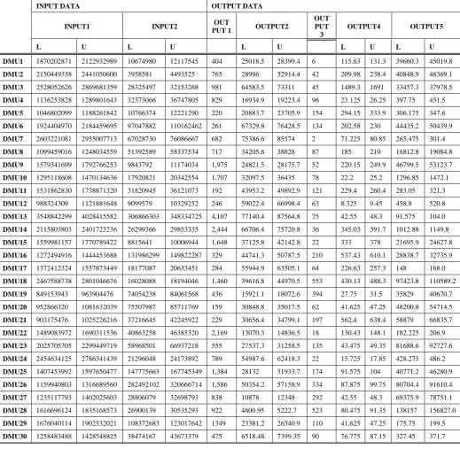
5. Numerical Example:

In this paper, the performance of electronic services in 30 branches of the Refah bank in 1389 will

be assessed. Variables will be introduced in terms of two inputs and five outputs and then using the

interval Balance index method and interval topsis, the data will be solved in the form of gams software.

And then after obtaining the upper and lower limits for the offered model, using the method mentioned

in Jahanshahloo and colleagues, paper in 2009, Bank branches will be ranked.

Table 1:

The data of the inputs and outputs

INPUT DATA OUTPUT DATA

INPUT1 INPUT2 OUT

PUT 1 OUTPUT2

OUT PUT 3

OUTPUT4 OUTPUT5

L U L U L U L U L U

DMU1 1870202871 2122932989 10674980 12117545 404 25018.5 28399.4 6 115.63 131.3 39660.3 45019.8 DMU2 2150449338 2441050600 3958581 4493525 765 28996 32914.4 42 209.98 238.4 40848.9 46369.1 DMU3 2528052626 2869681359 28325497 32153268 981 64583.5 73311 45 1489.3 1691 33457.3 37978.5 DMU4 1136253828 1289801643 32373066 36747805 829 16934.9 19223.4 96 23.125 26.25 397.75 451.5 DMU5 1046802099 1188261842 10766374 12221290 220 20883.7 23705.9 154 294.15 333.9 306.175 347.6 DMU6 1924404970 2184459695 97047882 110162462 261 67329.8 76428.5 134 202.58 230 44435.2 50439.9 DMU7 2603221081 2955007713 67028730 76086667 682 75386.6 85574 2 71.225 80.85 265.475 301.4 DMU8 1099459016 1248034559 51392589 58337534 717 34205.6 38828 87 185 210 16812.8 19084.8 DMU9 1579341699 1792766253 9843792 11174034 1,975 24821.5 28175.7 52 220.15 249.9 46799.5 53123.7 DMU10 1295118608 1470134636 17920821 20342554 1,707 32097.5 36435 78 22.2 25.2 1296.85 1472.1 DMU11 1531862830 1738871320 31820945 36121073 192 43953.2 49892.9 121 229.4 260.4 283.05 321.3 DMU12 988324309 1121881648 9099579 10329252 246 59022.4 66998.4 63 8.325 9.45 458.8 520.8 DMU13 3548842299 4028415582 306866303 348334725 4,107 77140.4 87564.8 75 42.55 48.3 91.575 104.0 DMU14 2115803803 2401723236 26299366 29853335 2,444 66706.4 75720.8 36 345.03 391.7 1012.88 1149.8 DMU15 1559981157 1770789422 8815641 10006944 1,648 37125.8 42142.8 22 333 378 21695.9 24627.8 DMU16 1272494916 1444453688 131986299 149822287 329 44741.3 50787.5 210 537.43 610.1 28838.7 32735.9 DMU17 1372412324 1557873449 18177087 20633451 284 55944.9 63505.1 64 226.63 257.3 148 168.0 DMU18 2467588738 2801046676 16028088 18194046 1,460 39616.8 44970.5 553 430.13 488.3 97423.8 110589.2 DMU19 849153943 963904476 74054238 84061568 436 15921.1 18072.6 394 27.75 31.5 35829 40670.7 DMU20 952866320 1081632039 75507987 85711769 159 30848.8 35017.5 62 41.625 47.25 48200.8 54714.5 DMU21 903175476 1025226216 37216645 42245922 229 30656.4 34799.1 197 562.4 638.4 58879 66835.7 DMU22 1489083972 1690311536 40863258 46385320 2,169 13070.3 14836.5 18 130.43 148.1 182.225 206.9 DMU23 2025705705 2299449719 58968501 66937218 555 27537.3 31258.5 135 43.475 49.35 81688.6 92727.6 DMU24 2454634125 2786341439 21296048 24173892 789 54987.6 62418.3 22 15.725 17.85 428.275 486.2 DMU25 1407453992 1597650477 147775663 167745349 1,384 28132 31933.7 174 91.575 104 40771.2 46280.9 DMU26 1159940803 1316689560 282492102 320666714 1,586 50354.2 57158.9 334 87.875 99.75 80704.4 91610.4 DMU27 1235117793 1402025603 28806079 32698793 838 10878 12348 292 42.55 48.3 69375.9 78751.1 DMU28 1616696124 1835168573 26900139 30535293 922 4600.95 5222.7 523 80.475 91.35 138157 156827.0 DMU29 1676040114 1902532021 108372683 123017642 1349 23381.2 26540.9 110 41.625 47.25 175.75 199.5 DMU30 1258483488 1428548825 38474167 43673379 475 6518.48 7399.35 90 76.775 87.15 327.45 371.7

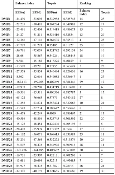
Finally, the upper and lower bounds obtained from solving model and the final

Table 2:

Final ranking of DMUs

Balance index Topsis Ranking

EFF(u) EFF(l) EFF(u) EFF(l) Balance

6. Conclusion

In this paper, we have proposed the ranking results by using 2 methods. As the following methods

have the different indexes for ranking, the results are different.

For example, when we use TOPSIS Method, the selected alternative should have the shortest distance

from the ideal solution and the farthest distance from the negative-ideal solution but in Balance Index

Method, each of the DMUs are evaluating according to their own weights and the others’.

So, the results are different because of the differences of the methods.

References

[1] M.R. Alirezaee, M.Afsharian, A and AR-IDEA: Models for dealing with imprecise data in DEA

models, Applied Mathematics and Computation 189 (2007) 1550–1559.

[2] R.D. Banker, A. Charens, W.W. Cooper, Some models for estimating technical and scale

inefficiencies in Data Envelopment Analysis, Management Science, 30 (1984) 1078-1092.

[3] A. Charnes, W.W. Cooper, E. Rodes, Measuring the efficiency of decision making units, European

Journal of Operational Research, 2 (6) (1978) 429-444.

[4] W.W. Cooper, K.S. Park, G. Yu, IDEA and AR-IDEA: Models for dealing with imprecise data in

DEA, Management Science 45 (1999) 597–607.

[5] M.J. Farrell, The measurement of productive efficiency, Journal of the Royal Statistical Society,

Series A, General 120 (3) (1957) 253-281.

[6] F. HosseinzadehLotfi, G R. Jahanshahloo, F. Rezaibalf, H. ZhianiRezai, Ranking of DMUs on

Interval Data by DEA, International Mathematical Forum, 2(4) (2007) 159-166.

[7] G.R. Jahanshahloo, F. HosseinzadehLotfi, A.R.Davoodi ,Extension of TOPSIS for decision-making

problems with interval data: Interval efficiency, Mathematical and Computer Modelling, 49, (2009)