Speech Enhancement using Gaussian Mixture Models,
Explicit Bayesian Estimation and Wiener Filtering
S. Chehrehsa* and M. H. Savoji**(C.A)
Abstract: Gaussian Mixture Models (GMMs) of power spectral densities of speech and noise are used with explicit Bayesian estimations in Wiener filtering of noisy speech. No assumption is made about the nature or stationarity of the noise. No Voice Activity Detection (VAD) or any other means is employed to estimate the input SNR. The GMM mean vectors are used to form sets of over-determined system of equations whose solutions lead to the first estimates of speech and noise power spectra. Based on the selected noise model from the initial noise power spectrum estimate, the noise source type is identified and the input SNR estimated in this first step. The first power spectra estimates are then refined using approximate but, explicit MMSE and MAP estimation formulations. The refined estimates are then used in a Wiener filter to reduce noise and enhance the noisy speech. The proposed filtering schemes show good results. Nevertheless, it is shown that the MAP explicit solution, introduced here for the first time, reduces the computation time to less than one third in comparison to the MMSE solution. Slight higher improvements in SNR and PESQ score and less distortion are also noted.
Keywords: Bayesian Estimation, GMM, MAP Solution, MMSE, Wiener Filtering.
1 Introduction1
Nowadays, the vast use of mobile communication in different environments with different background noises, asks for powerful and accurate noise reduction algorithms to ensure the quality of communicated voice and the performance of coding algorithms. Wiener filter is vastly used for noise reduction due to its simplicity. The performance of the Wiener filter is hinged on the accuracy of estimation of speech and noise Power Spectral Densities (PSDs). We proposed a codebook constrained Wiener filtering algorithm in which we solved a set of over-determined equations on codebook elements representing speech and different noise PSDs [1, 2]. The modeling by examples was used. Codebooks were created by clustering the PSDs of speech and noise signals of a training data-base using the k-means algorithm. No mathematical modeling was involved. To attain good results with the codebook constrained method we needed to use large codebooks resulting in long processing times. In fact, despite obtaining very good results, the processing time remained an issue. In the algorithm outlined in [3] we used mathematical
Iranian Journal of Electrical & Electronic Engineering, 2014. Paper first received 11 Jun. 2013 and in revised form 1 Feb. 2014. * The Author is with the School of Engineering, AUT University, Auckland, New Zealand.
** The Author is with the Faculty of Electrical and Computer Engineering, Shahid Beheshti University, Tehran, Iran.
E-mails: [email protected] and [email protected].
modeling, in the form of Gaussian Mixture Models (GMMs), for speech and noise PSDs. We solved over-determined sets of equations involving the GMM mean vectors to estimate speech and noise PSDs to form the Wiener filter used to enhance the noisy signal with almost the same performance but much less computation time. To further reduce the processing time we took advantage of the GMM mean vectors, to model the space of the input noisy PSDs, in a different manner in [4]. The observation vector corresponding to the noisy input was projected onto the mean vectors of the speech and different noise models to form again an over-determined set of equations whose solution led to the estimates of speech and noise PSDs and the input SNR. In [5], we showed that better results are obtained with models based on an approximate but explicit MMSE Bayesian estimation at a higher computation time which remains nevertheless low enough for practical implementations. In fact, the algorithm used in [4] to model the space spanned by the input noisy power spectra is employed in [5] to form the first estimates of speech and noise PSDs that are subsequently refined by the explicit MMSE estimations.
In this paper, we further improve our explicit Bayesian estimation using an explicit MAP solution derived from the previously used approximate MMSE formula. It is shown that better results are obtained at a much reduced processing time in comparison to the MMSE solution. The paper is organized as follows: In
section 2 we describe the Gaussian mixture modeling process used. In section 3, the Wiener filtering and its MMSE nature are outlined. In section 4, we state the explicit MMSE Bayesian estimation. Section 5 is the main concentration of this paper where we propose an explicit formula for implementing the MAP Bayesian estimation extracted from the MMSE formulation. In section 6, we describe our experiments and the measures used in evaluating the results discussed by the same token. Section 7 contains the conclusion comparing our MMSE and MAP speech enhancement solutions.
2 Gaussian Mixture Modeling
A practical method for modeling the Probability Density Function (PDF) of an arbitrary signal space is to use a mixture of Gaussian PDFs [6] where a data point is associated with different probabilities to different components of the mixture. A GMM for a process P (taken as a vector) is defined as:
( )
(
)
1 1
; , , 1
K K
k k k k k
k k
f P p G P μ p
= =
=
∑
Σ∑
= (1)where f is the PDF, Gk(P; μk, Σk) denotes the Gaussian
PDF of the k-th component of the mixture, with mean vector μk and covariance matrix Σk. The parameter pk is
the prior probability of the k-th mixture and is interpreted as the expected fraction of the number of vectors P associated with that mixture. The sum of these prior probabilities adds up to 1. Vector P can represent the spectral magnitude or spectral power of a frame or segment of the noisy speech, speech or noise signal. The number of mixtures k for speech and noise is set by trial and error in general (k = 6 to 9 is usual for speech) and the well-known Expectation – Maximization (EM) algorithm is applied for the estimation of the parameters of the GMM using a training data.
As stated in [3], we used our previously developed tree structured codebooks of speech and different noise sources to initialize the EM algorithm. In fact, knowing the number of vectors that have fallen in each cluster, the codebook is searched to find the k most populated clusters. Using the relative populations, mean vectors (centroids) and covariance matrices of these clusters as initial values, the EM algorithm is run on the whole training data to form the models. On the basis of some elementary results k = 6 and 9 were chosen for speech and noise signals, respectively.
Using a diagonal covariance matrix is not readily justified. Indeed the covariance matrix of the Babble noise, for instance, suggests strong correlation between spectral magnitudes or PSDs at neighboring frequencies due, in general, to frequency leakage resulting from windowing. The convergence problems of Gaussian mixture modeling, encountered when dealing with long vectors, are noted here as our spectral magnitudes and/or densities are calculated using 257 frequency bins.
3 MMSE Noise Reduction using Wiener Filter The MMSE criterion is widely used in speech enhancement. Such a solution is provided by Wiener filtering where estimates of the PSDs of speech and noise are used to modify the magnitude of the Short Time Fourier Transform (STFT) of the noisy signal which is then added to its unaltered phase characteristic. The Inverse Fourier Transform (IFFT) of this short time spectrum calculated usually, for overlapping segments of some 20-30 ms long, leads to the reconstruction of the filtered signal as output of the Overlap Add or Overlap Save algorithm. Assuming noisy signal in frequency domain as:
( ) ( ) ( )
X ω =S ω +N ω (2)
in which S(ω) and N(ω) are the FFT of the clean speech and noise respectively, a filter W(ω) is used, in Wiener filtering, to extract S(ω) from X(ω) as in:
ˆ( ) ( ) ( )
S ω =W ω X ω (3)
ˆ( )
S ω is the estimate of S(ω). It is well known that the MMSE between Sˆ( )ω and S( )ω is obtained when the Wiener filter defined below is applied:
( ) ( )
( ) ( )
s
s n
P W
P P
ω ω
ω ω
=
+ (4)
The Bayesian estimates of the PSDs of speech and noise signals may be used for Ps(ω) and Pn(ω). In [5]
we used the MMSE estimates as formulated in [7]. This formulation, repeated here in section 4 below, leads to our MAP formula derived in section 5.
4 MMSE Estimation of Speech and Noise PSDs Using the Gaussian mixture models containing the parameters pk, μk(ω) and Σk we can estimate Ps(ω) and
Pn(ω) to construct the suitable Wiener filter which is
subsequently used to enhance the noisy speech segment. As mentioned in [7] we know that the MMSE estimate of the PSD of the clean speech signal is calculated as:
[
|]
( | )MMSE
s s x s s s x s
P =E P P =
∫
P f P P d P (5) where fs refers to the PDF of the speech PSD given theobservation Px. It is derived, using the Bayesian
formula, as:
( | ) ( ) ( | )
( )
s x s s s
s s x
s x
f P P f P f P P
f P
= (6)
Combining f P Ps( |s x)and MMSE s
P we can write: ( | ) ( )
( | ) ( )
s s x s s s s
MMSE s
s x s s s s
P f P P f P d P P
f P P f P d P
=
∫
∫
(7)Using the GMMs of speech and noise, expressed in Eq. (1), we have:
6 6
1 1
9 9
1 1
( ) ( ; , ) , 1
( ) ( ; , ) , 1
i i i i i
j j j j j
s s s s x s s s
i i
n n n n x n n n
j j
f P p G P p
f P p G P p
μ
μ
= =
= =
= Σ =
= Σ =
∑
∑
∑
∑
(8)Here fn shows obviously the PDF of the noise PSD
also modeled with a Gaussian mixture. As stated earlier, the covariance matrices calculated by the EM algorithm are not diagonal, reflecting correlations among the low frequency bins of the PSDs. However, covariance vectors are used in [7] to calculate PDFs which means all estimations are calculated neglecting these correlations and approximating the covariance matrices as diagonal. Hence, we replace all Σk by σk which
represent the diagonals of the covariance matrices. By substituting Eq. (8) in Eq. (7) and using Gamma distribution we have as shown in [7]:
(
)
(
)
6 9
2 , , , 1 1
6 9
1 , , , 1 1 , , , , j i i j j i i j n s
i j i j i j
i j s n
MMSE s
n s
i j i j i j
i j s n
p p
I b c d P
p p
I b c d
σ σ σ σ = = = = =
∑∑
∑∑
(9)The elements of this equation are expressed as follows: 2 2 2 , , , 2 2 , , 4 1 , 4 4 2 ( 1 0
1 1 1
, ,
2
( )
1 ,
2
, e 1 erf ,
2
2 2
e e 1 erf ,
2 2 2
e
j i
i j i j
j i i j i x n s
i j i j
s n s n
x n s i j s n z i j i j z z b v v s P b c P d c z z D b z D z I P μ μ
σ σ σ σ
μ μ σ σ π π π − − +∞ − − ⎛ ⎞ ⎛ − ⎞ ⎜ ⎟ ⎜ ⎟ = + = − + ⎜ ⎟ ⎜ ⎟ ⎝ ⎠ ⎝ ⎠ ⎛ − ⎞ ⎜ ⎟ = + ⎜ ⎟ ⎝ ⎠ ⎧ ⎛ ⎞⎫ = = ⎨ − ⎜ ⎟⎬ ⎝ ⎠ ⎩ ⎭ ⎧ ⎡ ⎛ ⎞⎤⎫ ⎪ ⎪ = ⎨ − ⎢ − ⎜ ⎟⎥⎬ ⎝ ⎠ ⎣ ⎦ ⎪ ⎪ ⎩ ⎭ =
∫
( )
( )
( )
2 , , 2 , ) 4 2 ,e 2 e
j s i j s i j
i j
P c P d
s z v d
i j v
d P
b v D z
− − − − − = Γ (10)
Since our models are all normalized (the PSDs used are power normalized to one), they must be scaled according to the input SNR before being used. This is done using an estimate of the noise power in the following way. As we extract our input frames using Hamming windows with 75 % overlap, each processed frame is overlapped with three next and three previous frames. Assuming that the noise source power is almost unchanged in successive frames, we can assume that the noise power in the current frame is equal to the average power of the previous seven frames. Furthermore, assuming that the first few frames are silent and include just the environment noise, the noise power can easily be estimated using these frames at the beginning and be used as a good initial value for the averaging process of the next frames. If we consider the average noise power in the previous seven frames gn, equaling the noise
power in the current frame, the power of speech in the same frame or gs is estimated by removing gn from the
power of the noisy speech simply as:
( )
s x n
g P g
ω ω
=
∑
− (11)Therefore, for the purpose of scaling, all mean and covariance vectors in Eq. (10) are replaced using Eq. (11), as below:
2 2
, ,
i i i i
i i i i
s s s n n n
s s s n n n
g g
g g
μ μ μ μ
σ σ σ σ
→ →
→ → (12)
We note that we can construct the wiener filter using Eq. (9) in two ways. First, we can use the estimated
MMSE s
P to estimate MMSE n
P as MMSE MMSE
n x s
P =P −P (zeroing the eventual resulting negative values). Second, we can directly estimate MMSE
n
P using Eqs. (9-12) reversing the role of speech and noise by replacing μsi
and σsi with μnj and σnj and vice versa. This way the
two estimates MMSE s
P and MMSE n
P are not directly linked and therefore reflect better their assumed independence.
We have six different noise source candidates whose models must be used for the estimation of MMSE
s
P and
MMSE n
P for each noisy speech frame. To alleviate the computation we use the method exposed in [4], using speech and noise mean vectors to model the space of the noisy speech PSD, as a preprocessing step to find the suitable noise model i.e. the best noise candidate. Therefore, the following processing is limited to a single noise source. On the other hand, it is noted that the enhancement results using the spectral magnitude corresponding to the frame MMSE
s
P , directly attached to the noisy phase component of the same segment are poor. Therefore, MMSE
s
P and MMSE n
P estimates are used to construct the Wiener filter and carry out the enhancement by applying it to the noisy speech frame.
As could be seen from Eq. (10), the calculations of bi,j, ci,j and di,j involve using σsi and σnj in denominators. These occasionally very small values, mainly at high frequency components, result in large unwanted values for bi,j, ci,j and di,j. Poor estimations
result when summing them up in Eq. (9). Hence, we use a threshold and set the components less than a relatively small value, say ε, equal toε. In our reported results in Table 1 we use ε = 10-6.
5 Approximate MAP Solution
The noisy input phase is in fact the Maximum A-Posteriori (MAP) estimate of the clean speech phase and it is therefore more appropriate to combine the map estimate of the speech magnitude with this phase estimate to reconstruct the enhanced speech signal. It is expected that such a solution leads to better results. Different solutions based on different assumptions, approximations and/or methods have been suggested [8-11]. It is noted that MMSE and MAP solutions are Bayesian estimates that become equivalent to the Maximum Likelihood (ML) solution for symmetric distributions [6].
However, a true MAP solution may involve costly optimization algorithms that require good initializations to guarantee global optimum solution and acceptable speed of convergence. This was our initial interest in seeking a fast MMSE solution using GMM as initialization to an optimization algorithm. However, in the case of GMM an explicit MAP solution can be attained, as explained below, avoiding the use of optimization procedures. The MAP solution is obtained as:
arg max ( | ) ( )
s
MAP
s s x s s s
P
P = f P P f P (13)
Using fn(Pn) referring to the GMM of noise we have:
arg max ( ) ( )
s
MAP
s n x s s s
P
P = f P −P f P (14)
As previously stated an explicit formula for MMSE s
P
is suggested in [7] and put in practical use in [12]. This is while the vastly quoted paper of Ephraim and Malah introduces a different MMSE solution taking into account the probabilistic speech presence in a frame [13]. As shown in Eq. (13) we are looking for a speech PSD (Ps) that maximizes fs(Px|Ps)fs(Ps) expressed in the
denominator of Eq. (7). The first derivative of this denominator with respect to Ps is fs(Px|Ps)fs(Ps) whose
derivative (the second of the denominator) equated to zero, yields the sought Ps. Using Eqs. (7) and (9) we can
therefore write:
(
)
6 9
1 , , , 1 1 ( | ) ( ) , , j i i j
s x s s s s
n s
i j i j i j
i j s n
DEN f P P f P d P p p
I b c d
σ σ
= =
=
=
∫
∑∑
(15)where DEN stands for denominator. Knowing from Eq.
(10) that 2
1 0 exp( i j s, i j s, i j, ) s
I =
∫
+∞ −b P −c P −d d P the first derivative of Eq. (15) will be:(
)
2 , , , 6 9
1 , , ,
1 1 6 9 ( ) 1 1 ( | ) ( ) , , ( | ) ( ) e j i i j j
i i j s i j s i j
i j
s x s s s
s
n i j i j i j
s
i j s n s
s x s s s
s
n
s b P c P d
i j s n
DEN
f P P f P P
p I b c d p
P DEN
f P P f P P p p σ σ σ σ = = − − − = = ∂ = ∂ ∂ = ∂ ∂ = ∂ =
∑∑
∑∑
(16)Also, equating the second derivative of DEN to zero gives: 2 , , , 2 2 6 9 , , ( ) 1 1 ( | ) ( )
( 2 )
e 0
i j i j s i j s i j
i j
s x s s s
s s
s n i j s i j b P c P d
i j s n
f P P f P DEN
P P
p p b P c
σ σ − − − = = ∂ ∂ = ∂ ∂ − − =
∑∑
= (17)Now using the fact that, except for the last term, all the terms in the double summation are positive non zero values we can write:
2
, , ,
2 2
( )
6 9 6 9
, ,
1 1 1 1
e
( 2 )
i j s i j s i j
i j
i j
s
b P c P d
s n
i j s i j
i j i j s n
DEN P
p p b P c
σ σ − − − = = = = ∂ ≤ ∂ − −
∑∑
∑∑
(18)Requiring that 6 9 , , 1 1
( 2 i j s i j) 0
i j
b P c
= =
− − =
∑∑
, yields:6 9 , 1 1 6 9 , 1 1 2 i j i j MAP s i j i j c P b = = = = − =
∑∑
∑∑
(19)Alternative factorization of Eq. (19) leads to alternative solutions such as:
6 9 , 1 1 6 9 , 1 1 2 j i i j j i i j n s i j
i j s n
MAP s
n s
i j
i j s n
p p c P p p b σ σ σ σ = = = = − =
∑∑
∑∑
(20)The difference in these formulations is reflected in the slope of the derivative approaching zero. Our experiments show that almost the same results are obtained, on the average, using these different formulations. They all are slightly higher in terms of the achieved enhancement as compared to the MMSE solution as can be seen below. On the other hand, the MAP solution is also interesting because it reduces the computation time by avoiding the integration involved in the MMSE estimation. It is noted that the filter is again constructed using MAP estimates of both speech and noise. It is noted that, here also, the same scaling of the models is needed and applied. Again the best noise candidate is chosen, for each frame, as previously mentioned. Next section summarizes the results.
6 Experiments
The noise database is formed by 6 long files of babble, white, pink, destroyer engine, factory and HF channel noise. Each noise file contains more than 1.8 million samples and each clean speech file contains around 30000 to 60000 samples. The noise files are converted from 16 kHz originally to 8 kHz from NOISEX database available from the Rice University Digital Signal Processing (DSP) group home page [14]. The speech files are also quantized with 16 bit and have the sampling rate of 8 kHz extracted randomly from the TIMIT database [15]. These databases are divided into two parts. One is used to train the GMM models while the other is used to perform the speech enhancement tests. Hence the speech and noise files used for test are not present in the construction of the models. The MATLAB software is used on a Widows 64 bit based PC with Core i5 3.2 GHz CPU and 16 GB RAM for all simulations and tests. The test files are used to create noisy observations at -5, 0, 3, 5 and 10 dB input SNRs.
To test the mentioned algorithms, 50 speech files consisting of male and female speakers are used. The results shown in the table are averaged over the used files. Overlapping windowed (Hamming) segments of length of 256 samples (of 75% overlap) are used. The enhancement is calculated in terms of SNR and segmental SNR improvements. To calculate the SNR improvement we use the following:
( ) ( )
(
)
( ) ( )
(
)
2 2 10 log
ˆ
t
t
x t s t SNR imp
s t s t
⎛ − ⎞
⎜ ⎟
= × ⎜ ⎟
−
⎜ ⎟
⎝ ⎠
∑
∑
(21)x(t) is the noisy speech while ˆ( )s t and s(t) refer to the enhanced and clean speech respectively. We calculate the segmental SNR as:
( )
( )
(
)
( )
( )
(
)
2
2 1
10 log
ˆ
n n
N t seg
n n n
t
x t s t SNR imp
N = s t s t
⎛ − ⎞
⎜ ⎟
= ⎜ ⎟
−
⎜ ⎟
⎝ ⎠
∑
∑
∑
(22)Here, n refers to the n-th segment of the signal in the time domain. The segment length, in this calculation, is
one third of that used for noise reduction. Another measure used in the evaluation of results is distortion (in percentage). To calculate the distortion we use:
( ) ( )
(
)
( )
22
ˆ distortion 100 t
t
s t s t s t
−
= ×
∑
∑
(23)PESQ (Perceptual Evaluation of Speech Quality) value (0.5–4.5) is also used in our evaluations. PESQ is a quantitative psycho-acoustic measure that is used to evaluate how the enhanced speech is appreciated. To calculate PESQ as explained in [16], the routine available in [17] is used.
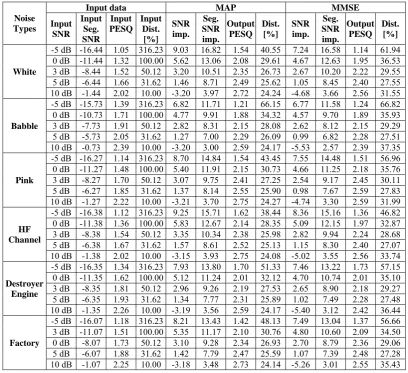
For the speech and noise PSD estimation part of the enhancement procedure using MMSE method, the algorithm mentioned in section 4 and [7] is used. For the proposed MAP method the algorithm in section 5 is used. The results of our experiments and the comparison of our proposed MAP method with the MMSE method are shown in Table 1 and illustrated in Figs. 1 and 2.
Table 1 Comparison of enhancement results using Bayesian estimation based on MAP and MMSE criterion.
Noise Types
Input data MAP MMSE
Input SNR
Input Seg. SNR
Input PESQ
Input Dist.
[%] SNR imp.
Seg. SNR imp.
Output PESQ
Dist. [%]
SNR imp.
Seg. SNR imp.
Output PESQ
Dist. [%]
White
-5 dB -16.44 1.05 316.23 9.03 16.82 1.54 40.55 7.24 16.58 1.14 61.94 0 dB -11.44 1.32 100.00 5.62 13.06 2.08 29.61 4.67 12.63 1.95 36.53
3 dB -8.44 1.52 50.12 3.20 10.51 2.35 26.73 2.67 10.20 2.22 29.55
5 dB -6.44 1.66 31.62 1.46 8.71 2.49 25.62 1.05 8.45 2.40 27.55
10 dB -1.44 2.02 10.00 -3.20 3.97 2.72 24.24 -4.68 3.66 2.56 31.55
Babble
-5 dB -15.73 1.39 316.23 6.82 11.71 1.21 66.15 6.77 11.58 1.24 66.82
0 dB -10.73 1.71 100.00 4.77 9.91 1.88 34.32 4.57 9.70 1.89 35.93
3 dB -7.73 1.91 50.12 2.82 8.31 2.15 28.08 2.62 8.12 2.15 29.29
5 dB -5.73 2.05 31.62 1.27 7.00 2.29 26.09 0.99 6.82 2.28 27.51
10 dB -0.73 2.39 10.00 -3.20 3.00 2.59 24.17 -5.53 2.57 2.39 37.35
Pink
-5 dB -16.27 1.14 316.23 8.70 14.84 1.54 43.45 7.55 14.48 1.51 56.96 0 dB -11.27 1.48 100.00 5.40 11.91 2.15 30.73 4.66 11.25 2.18 35.76
3 dB -8.27 1.70 50.12 3.07 9.75 2.41 27.25 2.54 9.17 2.45 30.11
5 dB -6.27 1.85 31.62 1.37 8.14 2.55 25.90 0.98 7.67 2.59 27.83
10 dB -1.27 2.22 10.00 -3.21 3.70 2.75 24.27 -4.74 3.30 2.59 31.99
HF Channel
-5 dB -16.38 1.12 316.23 9.25 15.71 1.62 38.44 8.36 15.16 1.36 46.82 0 dB -11.38 1.36 100.00 5.83 12.67 2.14 28.35 5.09 12.15 1.97 32.87
3 dB -8.38 1.54 50.12 3.35 10.34 2.38 25.98 2.82 9.94 2.24 28.68
5 dB -6.38 1.67 31.62 1.57 8.61 2.52 25.13 1.15 8.30 2.40 27.07
10 dB -1.38 2.02 10.00 -3.15 3.93 2.75 24.08 -5.02 3.55 2.56 33.74
Destroyer Engine
-5 dB -16.35 1.34 316.23 7.93 13.80 1.70 51.33 7.46 13.22 1.73 57.15 0 dB -11.35 1.62 100.00 5.12 11.24 2.01 32.12 4.70 10.74 2.01 35.10
3 dB -8.35 1.81 50.12 2.96 9.26 2.19 27.53 2.65 8.90 2.18 29.27
5 dB -6.35 1.93 31.62 1.34 7.77 2.31 25.89 1.02 7.49 2.28 27.48
10 dB -1.35 2.26 10.00 -3.19 3.56 2.59 24.17 -5.40 3.12 2.42 36.44
Factory
-5 dB -16.07 1.18 316.23 8.21 13.43 1.42 48.13 7.49 13.04 1.37 56.66 3 dB -11.07 1.51 100.00 5.35 11.17 2.10 30.76 4.80 10.60 2.09 34.50
0 dB -8.07 1.73 50.12 3.10 9.28 2.34 26.93 2.70 8.79 2.36 29.06
5 dB -6.07 1.88 31.62 1.42 7.79 2.47 25.59 1.07 7.39 2.48 27.28
10 dB -1.07 2.25 10.00 -3.18 3.48 2.73 24.14 -5.26 3.01 2.55 35.43
Fig. 1 The comparison of PESQ improvement using MMSE and MAP methods with respect to input PESQ.
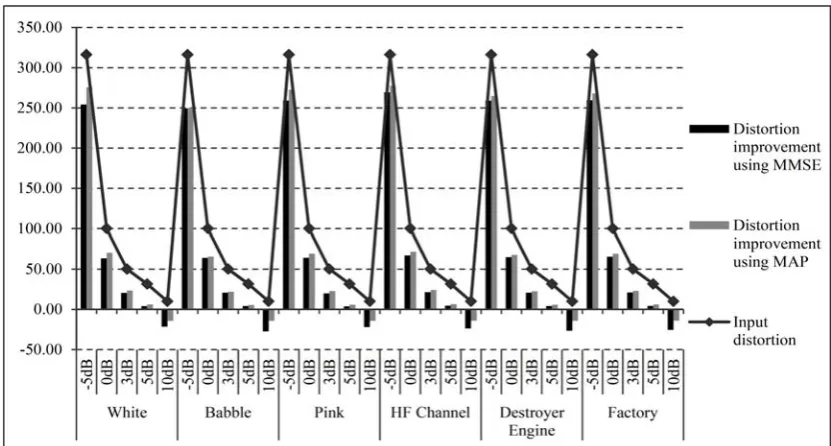
Fig. 2 The comparison of Distortion improvement using MMSE and MAP methods with respect to input distortion in percent.
As could be seen from Table 1 and Figs. 1 and 2, the proposed MAP method exhibits better results in terms of SNR, Segmental SNR and distortion improvements. This is due probably to the fact that the MMSE estimate is obtained by an average PDF function while maximum PDF is used in the MAP estimation. In fact, it is noticed that the MMSE estimation results in smoother estimated speech and noise PSDs. Estimated PSDs obtained in MAP estimation are somehow more ragged and sparse reflecting better the sparsity of PSDs in the frequency domain. It can also be seen, from Table 1 and Figs. 1 and 2, that for input SNR of 10 dB the SNR is decreased and the distortion increased using either MAP or MMSE
estimates. This is while segmental SNR and PESQ are increased. It is noted, generally speaking, that speech is highly non stationary and segmental SNR and PESQ reflect better the performance of the algorithms than SNR and distortion measures calculated as averages on the whole signal length. On the other hand, the quality of the 10 dB signal is already high and the used models do not reflect the sharpness encountered in the high quality speech signal so that applying the Wiener filter is not beneficial, in terms of all measures, in this case. Our investigation showed that for high SNR inputs more refined models (higher number of clusters) must be used.
From Table 1 and Fig. 1 we can see that in most cases, the MAP algorithm exhibits higher segmental SNR improvement, PESQ and lower distortions than MMSE algorithm except for -5 and 0 dB input SNRs of Babble noise where the PESQ improvements are almost the same. In fact, Babble noise is speech-like, making filtering, at these low SNRs, a difficult task. Actually, there might be confusion in distinguishing between speech and noise for some frames. Lower PESQ improvements are noted in 0, 3 and 5 dB input SNR in the case of Pink noise when comparing these results. Here, the low energy unvoiced frames, whose power spectra are similar to the long term PSD of Pink noise, are unduly suppressed in the filtering process.
The most important difference in using MAP as compared to the MMSE algorithm is the processing time. The average processing time of a file was almost 5 Sec for the MMSE algorithm while it was just 1 Sec in case of MAP.
7 Conclusion
The MAP solution, based on an explicit formulation introduced in this paper, yields higher PESQ and segmental SNR improvement and also less distortion in comparison to the MMSE method for almost all noise types and input SNRs. This relatively good performance is, however, more noted when the lower complexity and lower process time of this solution are taken into account. In fact the mean process time for each file using MAP is one fifth of the MMSE method. It is noted that both solutions result in much lower distortions than our previous methods [3] and [4]. The lower distortion is better appreciated in informal listening than reflected in PESQ or segmental SNR improvement.
We emphasize that we used, in this paper, an explicit MMSE formula to estimate speech and noise PSDs, independently, which were then used in the construction of the Wiener filter. We also transformed this explicit MMSE formula to express an explicit formula for the MAP estimations of our speech and noise PSDs. By doing so we proposed a solution which achieves almost the same results at a much reduced processing time. Our future line of work includes, among other things, comparison of our MAP solution with a solution based on using optimization algorithms albeit at a much higher computation time. This comparison is interesting in the sense that it should shed some light on the relevance of the orthogonal assumption made here on the covariance matrices of the Gaussian mixture models.
References
[1] S. Chehresa and M. H. Savoji, “Codebook Constrained Iterative and Parametric Wiener Filter Speech Enhancement”, in IEEE International Conference on Signal and Image Processing Applications (ICSIPA), Kuala Lumpur, pp. 548-553, Nov. 2009.
[2] S. Chehresa and M. H. Savoji, “Improved Codebook Constrained Wiener filter Speech Enhancement”, in 5th International Symposium on
Telecommunications, Tehran, pp. 614-618, Dec. 2010.
[3] S. Chehresa and M. H. Savoji, “MMSE speech enhancement based on GMM and solving an over-determined system of equations”, IEEE 7th
International Symposium on Intelligent Signal Processing (WISP), Floriana, pp. 1-5, Sep. 2011. [4] S. Chehresa and M. H. Savoji, “Speech
enhancement based on Gaussian Mixture Modeling and Wiener filtering”, International Journal on Communications Antenna and Propagation (I.Re.C.A.P), Vol. 2, No. 2, pp. 111-122, Apr. 2012.
[5] S. Chehresa and M. H. Savoji, “MMSE speech enhancement using GMM”, 16th CSI
International Symposium on Artificial Intelligence and Signal Processing (AISP), Shiraz, pp. 266-271, May 2012.
[6] S. Vasseghi, Advanced Digital Signal Processing and Noise Reduction, Wiley, West Sussex, England, 2006.
[7] I. Potamitis, N. Fakotakis, N. Liolios and G. K. Kokkinakis, “Speech Enhancement Using Mixtures of Gaussians for Speech and Noise”, 5th
Text, Speech and Dialogue Conference, pp. 337-340, 2002.
[8] D. Burshteinand and S. Gannot, “Speech Enhancement Using a Mixture-Maximum Model”, IEEE Transaction on Speech and Audio Processing, Vol. 10, No. 6, pp. 341-351, Sep. 2002.
[9] T. Lotter and P. Vary, “Speech Enhancement by MAP Spectral Amplitude Estimation Using a Super-Gaussian Speech Model”, EURASIP Journal on Applied Signal Processing, pp. 1110-1126, Jan. 2005.
[10] A. Kundu, S. Chatterjee, A. Sreenivasa Murthy and T.V. Sreenivas, “GMM Based Bayesian Approach To Speech Enhancement In Signal Transform Domain”, IEEE International Conference on Acoustics, Speech and Signal Processing (ICASSP), pp. 4893-4896, Mar. 2008. [11] J. Hao, T. Lee and T. J. Sejnowski, “Speech
Enhancement Using Gaussian Scale Mixture Models”, IEEE Transaction on Audio, Speech, and Language Processing, Vol. 18, No. 6, pp. 1127-1136, Aug. 2010.
[12] T. Ganchev, I. Potamitis , N. Fakotakis and G. Kokkinakis, “Text-Independent Speaker Verification for Real Fast-Varying Noisy Environments”, International Journal of Speech Technology, Vol. 7, No. 4, pp. 281-292, Oct. 2004.
[13] Y. Ephraim and D. Malah, “Speech enhancement using a minimum mean square error short time amplitude estimator”, IEEE Transaction on Acoustic, Speech and Signal Processing, Vol. 32, No. 6, pp. 1109-1121, Dec. 1984.
[14] The Rice University, Signal Processing Information Base (SPIB) (1995), Noise data [Online], Available:
http://spib.rice.edu/spib/select_noise.html.
[15] J. Garofolo, L. Lamel, W. Fisher, J. Fiscus, D. Pallett, N. Dahlgren and V. Zue, (1993), TIMIT Acoustic-phonetic continuous speech corpus [Online], Available:
www.ldc.upenn.edu/Catalog/CatalogEntry.jsp?cat alogId=LDC93S1.
[16] Y. Hu and P. Loizou, “Evaluation of objective quality measures for speech enhancement”, IEEE Transactions on Audio, Speech and Language Processing, Vol. 16, No. 1, pp. 229-238, Jan. 2008.
[17] P. Loizou, NOIZEUS: A noisy speech corpus for evaluation of speech enhancement algorithms [Online], Available:
www.utdallas.edu/~loizou/speech/noizeus.
Sarang Chehrehsa was born in
Lahijan, Iran, 1983. He finished his M.Sc. in Electrical Engineering in Shahid Beheshti University, Iran, 2009 and his B.Sc. in Electrical Engineering in University of Guilan, Rasht, Iran, 2006. His research interests are, signal processing, speech enhancement, modeling and recognition. Currently he is pursuing Ph. D. in Auckland University of Technology (AUT), New Zealand. The focus of his Ph.D. is on the modeling of speech and noise PDF distribution and speech enhancement.
Mohammad Hassan Savoji was born in Tehran, Iran in 1949. He finished his B.Sc. and M.Sc. studies, in Electrical Engineering, in Sharif Technical University, Tehran in 1972 and 1975 respectively. He received his Ph.D. (Docteur-Ingenieur) from INPG (Institut National Polytechnique de Grenoble) in Electronics and Telecommunications in 1979. He carried out a post-doctorate in Oxford University in 1981. He worked at various European Universities and Research Centers between 1981 and 1995. His last appointment before returning to Iran was in Santander University, Spain, as Professor and Head of Signal Processing Group. Since 2001, he is Professor of Electronics and Telecommunications in Electrical and Computer Engineering Faculty of Shahid Beheshti University, Tehran, Iran. He has published more than 80 Journal and Conference papers on different aspects of Signal Processing. He also holds two patents. Some of his interests include Signal Processing, Image and Video Processing, Speech Processing, Adaptive and Non-linear Filters. Professor Savoji is a Chartered Engineer and has been a member of IEEE and IEE and has served, in the past, on the IEE C5 (Human Computer Interaction) Professional Group.