Analysing Student Performance using Sparse Data of Core Bachelor Courses

Analysing Student Performance using

Sparse Data of Core Bachelor Courses

Mirka Saarela

Tommi K ¨arkk ¨ainen

Curricula for Computer Science (CS) degrees are characterized by the strong occupational orientation of the discipline. In the BSc degree structure, with clearly separate CS core studies, the learning skills for these and other required courses may vary a lot, which is shown in students’ overall performance. To analyze this situation, we apply nonstandard educational data mining techniques on a preprocessed log file of the passed courses. The joint variation in the course grades is studied through correlation analysis while intrinsic groups of students are created and analyzed using a robust clustering technique. Since not all students attended all courses, there is a nonstructured sparsity pattern to cope with. Finally, multilayer perceptron neural network with cross-validation based generalization assurance is trained and analyzed using analytic mean sensitivity to explain the nonlinear regression model constructed. Local (within-methods) and global (between-(within-methods) triangulation of different analysis methods is argued to improve the technical soundness of the presented approaches, giving more confidence to our final conclusion that general learning capabilities predict the students’ success better than specific IT skills learned as part of the core studies.

Keywords: Sparse Educational Data, Triangulation, Curricula Refinement, Correlation Analy-sis, Robust Clustering, Multilayer Perceptron

[This version was updated August 19, 2015, for format revision]

1.

I

and personal attributes are important (Sahami et al., 2013a). For more than 40 years, roughly every 10 years, the Association for Computing Machinery (ACM) and the Institute of Electrical and Electronics Engineers (IEEE) have promoted the creation of international curricular guide-lines for bachelor programs in computing (Sahami et al., 2013b). Thus far, however, there has been little discussion about the relation between specific CS courses and other courses, in terms of the overall study performance.

Some researchers (see, e.g., Kinnunen et al. 2013and references therein) indicate that pri-marily difficulties in mastering programming lead to high dropout rates in CS, therefore, one should pay special attention to them. Furthermore, a popular belief is that mathematical talent is the key skill for CS students to be successful (Jerkins et al., 2013). Although these topics are important, they do not cover the whole degree. The CS core of the DMIT curriculum for undergraduate students at the University of Jyv¨askyl¨a, one of the largest and most popular mul-tidisciplinary universities in Finland, has been more or less the same in recent years. Since the curriculum is typically updated every three years, the aim of this research is to focus on a set of mandatory courses related to the data collection period August 2009 through July 2013.

In addition, DMIT undergraduate students require more time to finish their studies com-pared to students of other disciplines at the University of Jyv¨askyl¨a (Halonen, 2012). This happens even if the student’s view on the quality of teaching and the study atmosphere at DMIT Jyv¨askyl¨a is very positive and, in fact, better than in the whole Faculty of Information Tech-nology (of which the DMIT is a part) or in the other departments at the university (Halonen, 2012). Actually, only a very few students (on average12.8%) of DMIT complete the national target of at least 55 ECTS per academic year (Harden and Tervo, 2012). These study efficiency shortcomings apply to the absolute and relative number of credits and are especially important compared with students of other departments at the University of Jyv¨askyl¨a, who amass many more credits in an academic year (29%acquire at least 55 ECTS).

To assess the current curriculum, we apply the educational data mining (EDM) approach. EDM consists of developing or utilizing data mining methods that are especially feasible for discovering novel knowledge originating in educational settings (Baker and Yacef, 2009) and supporting decision-making in educational institutions (Calders and Pechenizkiy, 2012). Most of the current case studies in EDM (see Table1) analyze the steadily growing amount of log data from different computer-based learning environments, such asLearning Management Systems (e.g., Valsamidis et al. 2012), Intelligent Tutoring Systems(e.g., Hawkins et al. 2013;Bouchet et al. 2012; Carlson et al. 2013; Springer et al. 2013), or even Educational Games (e.g., Kerr and Chung 2012;Harpstead et al. 2013). Mining those data supports the understanding of how students learn and interact in such systems.

In our study, however, we are interested in understanding the effects of core CS courses and providing novel information for refining repetitive curricula. More specifically, we want to understand the effect of the current profile of the core courses on students’ study success. These courses are taught in an ordinary fashion, meaning that in order to successfully complete a course, the student has to attend lectures, complete related exercises, and pass a final exam or assignment at the end of the course. The data analyzed in this paper are the historical log file from the study database at DMIT about all courses students passed for the period August 20091 until the end of July 2013. Patterns in our data provide improved profiling of the core courses and an indication of which study skills support timely and successful graduation.

The remainder of this paper is structured as follows. In Section 2, the overall methodology is explained. Section3is devoted to the correlation analysis, while in Section4we discuss our clustering analysis with robust prototypes. In Section5, prediction analysis is realized with the multilayer perceptron (MLP) neural network. Conclusions from the domain as well as from the methodological level are presented in Section6.

2.

T

: A

-LATION

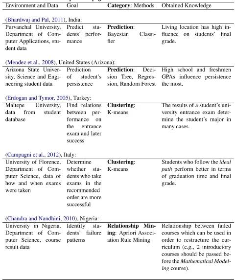
Baker et al.(2010) classify EDM methods into five categories: prediction, clustering, relation-ship mining, discovery with models, and distillation of data for human judgment. In Table1, we summarize a representative set of EDM studies according to a) their data and the environment, b) goal of the study, c) EDM category and methods, and d) the knowledge discovered. This work was selected from forums, such as the Journal of Educational Data Mining, related annual conferences, and Google Scholar during autumn 2013. According to the table, which is orga-nized by the different tasks and publication dates, scholars usually apply methods belonging to one of the classes of Baker et al.’s taxonomy to address a particular EDM problem. Moreover, predictive studies may apply many classifiers to assess the stability and reliability of the results. We, however, aim at multiphase triangulation: Different phases of the overall treatment within-methods and between-within-methods are varied and assessed (using rankings) to increase the technical soundness of the procedures and the overall reliability of the concluded results.

Generally, triangulation means that the same research objective is investigated by different data, theories, analysis methods, or researchers and then combined to arrive at convergent find-ings (Denzin, 1970). Probably the most popular way to apply triangulation is to use qualitative and quantitative methods and merge their results (Jick, 1979). We employ between-method triangulation (e.g., Denzin 1970; Bryman 2003), using techniques from distinct classes of the EDM taxonomy, to study the success patterns of the students who take the core courses of the computer science program in our department. First, we apply correlation analysis (Section 3), a key technique inrelationship mining. Second, we utilize a special clustering approach (see Section 4) to find groups of students with similar course success. Third, we applyprediction (see Section 5) with model sensitivity analysis. In all between-methods, we discuss different within-methodsthat tighten the soundness of the respective between-method result. Moreover, we support our decision making a) in clustering with thedistillation of data for human judgement (see our explorative and visual analysis in Section4.2.1) and b) in prediction withdiscovery with models(model sensitivity is used as a component to calculate the mean variable sensitivity of the prediction model; see Section5.1. To combine and interpret our results from the individual EDM techniques, we introduce a ranking system to which all the between and within analysis methods contribute.

Table 1: Overview of related work.

Environment and Data Goal Category: Methods Obtained Knowledge (San Pedro et al., 2013), United States (New York):

Interaction data of a web-based tutoring system for mathematics from 3747 middle school students in New England plus college enrollment information for the students

Predict

whether a student will (5 years later) attend college

Prediction: Logis-tic Regression Clas-sifier

Students who are successful in middle school mathemat-ics as measured by the tutor-ing system are more likely to enroll 5 years later in college, while students who are bored, confused, or careless in the system have a lower probabil-ity of enrolling.

(Vihavainen et al., 2013), Finland: Helsinki University,

snapshot data from Computer Science student programming course Predict whether a student will fail the in-troductory mathematics course Prediction: Non-parametric Bayesian network tool (B-Course)

Students who cram at dead-lines in their programming course are at high risk of fail-ing their introductory mathe-matics course.

(Bayer et al., 2012), Czech Republic: Masaryk University,

data of Applied In-formatics bachelor students, their studies, and their activities in the university’s information system (e.g., communication with other students via email/discussion board)

Predict

whether a bachelor stu-dent will drop out of the university

Prediction: J48 decision tree learner, IB1 lazy learner, PART rule learner, SMO support vector machines, NB

Students who communicate with students who have good grades can successfully grad-uate with a higher probabil-ity than students with similar performance but who do not communicate with successful students.

(Kotsiantis, 2012), Greece: Hellenic Open Univer-sity, data from distance learning course on In-formatics

Predict stu-dents’ final marks

PredictionM5’, BP, LR, LWR, SMOreg, M5rules

Two written assignments pre-dict the students’ final grade the best.

Table 1 – continued from previous page

Environment and Data Goal Category: Methods Obtained Knowledge

(Bhardwaj and Pal, 2011), India: Purvanchal University,

Department of Com-puter Applications, stu-dent data Predict stu-dents’ perfor-mance Prediction: Bayesian Classi-fier

Living location has high in-fluence on students’ final grade.

(Mendez et al., 2008), United States (Arizona): Arizona State

Univer-sity, Science and Engi-neering student data

Prediction of student’s persistence

Prediction: Deci-sion Tree, Regres-sion, Random Forest

High school and freshmen GPAs influence persistence the most.

(Erdogan and Tymor, 2005), Turkey: Maltepe University,

data from student database

Find relations between per-formance on the entrance exam and later success

Clustering: K-means

The results of a student’s uni-versity entrance exam deter-mine the student’s major in many cases.

(Campagni et al., 2012), Italy: University of Florence, Department of Com-puter Science, data of how and when exams were taken

Determine whether stu-dents who take exams in the recommended order are more successful

Clustering: K-means

Students who follow theideal path perform better in terms of graduation time and final grade.

(Chandra and Nandhini, 2010), Nigeria: University in Nigeria,

Department of Com-puter Science, course result data

Identify stu-dents’ failure patterns

Relationship Min-ing: Apriori Associ-ation Rule Mining

Relationship between failed courses which can be used in order to restructure the cur-riculum (e.g., 2 introductory courses should be passed be-fore theMathematical Model-ingcourse).

2.1. DATA AND NONSTRUCTURED SPARSITY PATTERN

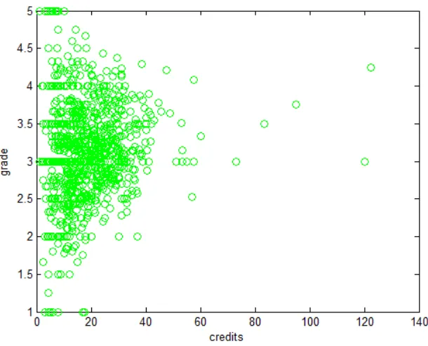
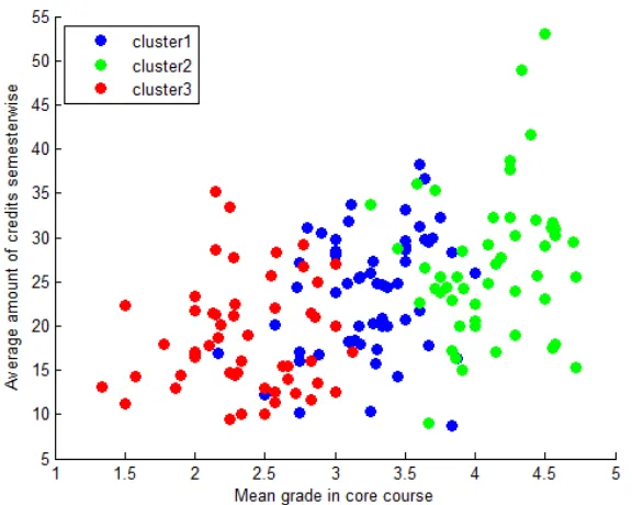
Figure 1: Relationship between the average credits per semester and grades.

have diverse interests, choose their optional courses accordingly, and, as a consequence, realize very different study profiles. This is a typical situation in multidisciplinary universities where students have the opportunity to choose from a large pool of courses. Altogether, our dataset consists of13640study records with21attributes, related to the passed course and the student’s affiliation, and of 1040 students who attended a total of 1271 different courses, completing a total of64905credits. Only64%of these credits the CS students obtained from courses in their own faculty.

When measuring the performance of individual students, in addition to quality, i.e., the grades, the quantity of studies, i.e., the number of all earned credits, is important. However, since our dataset consists of many students at different stages of their education, we cannot com-pare their individual sums of credits as is. Therefore, we assigned each passed course/record in our dataset to a semester, so that themean credits(i.e., the average number of credits per student per semester) over the active semesters could be computed for all students. An active semester, in turn, is computed as the sum of all semesters between the first semester and the last semester that a student successfully completed a course. For example, a student who passed his or her first course in April 2010 and his or her last course in June 2013 has 7active semesters. This may include semesters in which the student did not earn any credits. Themean gradeis simply the sum of all grades divided by the number of courses a particular student has passed.

Table 2: Core bachelor courses.

course name course code course type completion mode2 _credits Computer and Datanetworks as Tools PCtools introductory assignment 2-4 Datanetworks Datanet introductory exercises & final exam 3-5 Object Oriented Analysis and Design3 OOA&D professional exercises & final exam 3-6

Algorithms 1 Alg1 professional final exam 4

Introduction to Software Engineering IntroSE professional final exam 3 Operating Systems OpSys professional final exam 4 Basics of Databases and Data Management DB&DMgm professional final exam 4 Programming 1 Prog1 programming assigment & final exam 6 Programming 2 Prog2 programming assigment & final exam 8 Computer Structure and Architecture CompArc introductory exercises & final exam 3 Programming of Graphical User Interfaces GUIprog programming exercises & final exam 5 Research Methods in Computing CompRes methodological essay 2

All core courses 47-54

Our goal is to better understand the students’ success patterns, given the core courses, in re-lation to the rest of their studies. Therefore, we want to analyze the students who have completed a certain percentage of the courses of interest. The core courses, a specific set of12courses that, for that period of time we study, have been a mandatory part of the curriculum for all DMIT bachelor students, are listed and characterized in Table2.

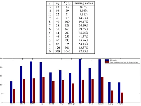
If we transform our data in such a way that the 12 core courses become the variables and the attribute value of each observation, corresponding to one student, is the grade of the core course ormissingif the student did not attend or pass the course, the assembled matrix is very sparse. Only for 13 students are the rows full; the students have passed all the core courses. In Table 3, the high percentage of missing values and the sparsity of the matrix are summarized. The table shows how many students have completed exactly, and respectively at least,q of the 12 courses. Moreover, in each case the percentage of missing values of the cumulative data matrix is provided. The missing data values in the matrix aremissing at random(Rubin, 1976; Rubin and Little, 2002). This means that the missing values are related to particular variables (some courses that are usually taken later in the program are completed by fewer students; see Figure2) but not missing because of the values (grades) that could be observed if a particular course is passed.

To analyze such data, one cannot accept too many missing values. In this respect, the break-down pointrelated to statistical estimates (see, e.g.,Hettmansperger and McKean 1998) on how much contamination (errors, missing values) in data can be tolerated is informative. An upper bound is easy to establish: If more than 50% of data is missing, then “missing” is the most typical value (mode) of the data. Furthermore, tests conducted with synthetic data show that,

2_{The difference betweenassignment and exercisesin our system is important: Whileassignment denotes a} mandatory work that the student has to fulfill in order to pass the course and affects the final grade the student will receive,exercisesare smaller (usually weekly) optional tasks that correspond to the current lecture material.

3_{In spring 2012, theObject Oriented Analysis and Design(OOA&D) course was split into two separate courses,}

Table 3: Number of students who have completed exactlyq(nq) or at leastq (PQq=12nq, Q =

12, . . . ,0) of the core courses during the analyzed period.

q nq Pnq missing values 12 13 13 0.0%

11 16 29 4.56%

10 22 51 9.81%

9 26 77 14.93%

8 49 100 19.17%

7 28 128 24.10%

6 35 163 29.65%

5 44 207 35.75%

4 46 253 41.37%

3 40 293 45.96%

2 82 375 54.13%

1 126 501 63.57%

0 539 1040 82.45%

Figure 2: Number of students who passed coursewise.

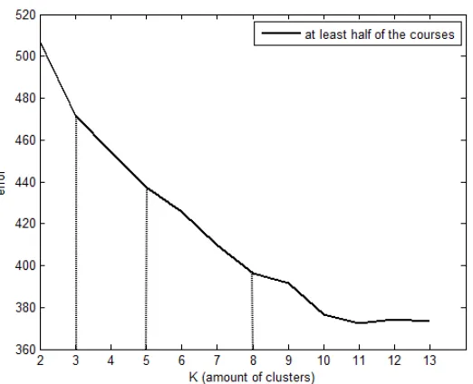
for example, in clustering with robust methods, reliable results, i.e., almost zero error, can be obtained even if around30%of the data is missing (Ayr¨am¨o 2006; see in particular Figure 22¨ at page 131). Therefore, ourdata selection strategyis to use that part of the whole, sparse data matrix, which contains the students who have completed at least half of the core courses. This dataset has about30%missing values (see Table3) for the multivariate techniques. In the cor-relation analysis (see Section3), where the courses are analyzed individually, we similarly use the subsets of the students who have passed the particular course and at least five other courses additionally. In addition, different subsets of the sparse study matrix are utilized to realize some parts of cluster analysis and predictive analysis procedures.

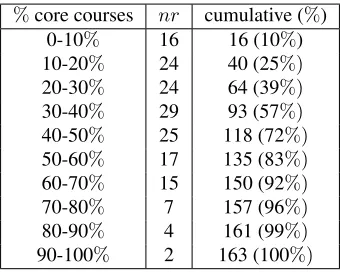
Table 4: Binning of students (nr= number) according to means of the number of core courses in relation to whole studies.

%core courses nr cumulative (%) 0-10% 16 16 (10%) 10-20% 24 40 (25%)

20-30% 24 64 (39%)

30-40% 29 93 (57%)

40-50% 25 118 (72%)

50-60% 17 135 (83%)

60-70% 15 150 (92%)

70-80% 7 157 (96%)

80-90% 4 161 (99%)

90-100% 2 163 (100%)

Summing up, for our analysis we have the entire base of completed courses (1040x21) that is processed and transformed to further subsets and the sparse163x12data matrix of the students who have completed at least half of the core courses and the grades they received in these courses.

3.

C

B

As our first EDM technique, we apply relationship mining using correlation analysis. In general, we know from Figure 1that in terms of grades well-scoring students are not necessarily more likely to study actively. But how about the correlation for our target group, those students who have already completed at least half of the core courses? In the correlation analysis, we do not need special methods for the sparse data. However, the number of students who have passed an individual course differs considerably (see Figure 2) so that the correlation coefficients are computed for different student subsets. The mean number of credits and the mean grade are computed in the same way as explained in Section2.1.

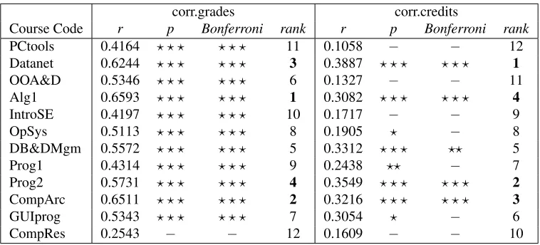
In Table 5, the correlation of each core course to (i) the mean grade of a student (denoted as corr.grades) and (ii) the mean number of credits per semester (denoted as corr.credits) is summarized. In each case, r identifies the calculated correlation, and p corresponds to the p-value for testing the hypothesis of no correlation, respectively. The number of stars indicates the strength of the evidence for no correlation. As usual, ? symbolizes the borderline to be significant(p <= 0.05),??symbolizesstatistically significant(p <= 0.01), and???symbolizes highly statistically significant(p <= 0.005). rankdenotes the ordering of courses by means of the computed correlations.

conserva-Table 5: Correlation of each core course to the students’ general performance.

corr.grades corr.credits

Course Code r p Bonferroni rank r p Bonferroni rank

PCtools 0.4164 ? ? ? ? ? ? 11 0.1058 − − 12 Datanet 0.6244 ? ? ? ? ? ? 3 0.3887 ? ? ? ? ? ? 1

OOA&D 0.5346 ? ? ? ? ? ? 6 0.1327 − − 11 Alg1 0.6593 ? ? ? ? ? ? 1 0.3082 ? ? ? ? ? ? 4

IntroSE 0.4197 ? ? ? ? ? ? 10 0.1717 − − 9 OpSys 0.5113 ? ? ? ? ? ? 8 0.1905 ? − 8 DB&DMgm 0.5572 ? ? ? ? ? ? 5 0.3312 ? ? ? ?? 5 Prog1 0.4314 ? ? ? ? ? ? 9 0.2438 ?? − 7 Prog2 0.5731 ? ? ? ? ? ? 4 0.3549 ? ? ? ? ? ? 2

CompArc 0.6511 ? ? ? ? ? ? 2 0.3216 ? ? ? ? ? ? 3

GUIprog 0.5343 ? ? ? ? ? ? 7 0.3054 ? − 6

CompRes 0.2543 − − 12 0.1609 − − 10

tive Bonferroni correction (Rice, 1989) that the correlation of all core courses to the student’s overall grade (except theResearch Methods in Computing) are highly statistical relevant.

Another conclusion that can be made from Table5is that the same four courses that have the highest correlations to the general success of the student also have the highest correlation to the average number of credits. This means that if a student gets a high grade in these courses he or she will probably earn, on average, a high number of credits in the semester as well. Again, all of these findings are, according to the classical p-test as well as the Bonferroni correction, highly statistically significant. Although the ranking is different (e.g., while Algorithm 1 correlates the most with the mean grade for the student,Datanetworkscorrelates the most with the mean number of credits per semester), we can conclude that those four courses correlate with the students’ general performance the best.

To sum up, it can be inferred that a student who achieves a high grade inAlgorithms 1, Com-puter Structure and Architecture,Datanetworks, orProgramming 2is likely to be successful in the remaining part of his or her studies not only with the grade level but also in terms of speed of completing courses. Albeit overall semesterwise credits and average grade do not correlate at all (see Figure1), a linear dependency between the grades a student received in the core courses and the general performance exists.

4.

C

Algorithm 1:Iterative relocation clustering algorithm Input: Dataset and the number of clustersK.

Output: Kpartitions of the given dataset. SelectKpoints as the initial prototypes; repeat

1. Assign individual observation to the closest prototype; 2. Recompute the prototypes with the assigned observations; untilThe partition does not change;

can be realized using the iterative relocation algorithm skeleton presented in Algorithm1with different score functions (Han et al., 2001) according to which the two steps inside the loop of Algorithm1are optimized.

However, in order to realize a prototype-based partitive clustering algorithm, two main is-sues should be addressed. First, a well-known problem of all iterative relocation algorithms is their initialization. They minimize the given score function locally by iteratively relocating data points between clusters until an optimal partition is attained. Therefore, basic iterative algorithms, such as K-means, always converge to a local, and not necessarily to the global, op-timum. Although much work has focused this problem, no efficient and universal method for identifying the initial partitions and the number of clusters exists. This problem is discussed more thoroughly in Section4.2. The second problem is the sparse student data with around 30% missing values (see Section2.1). In Section4.1, a solution is presented for adjusting the score function of the basic algorithm skeleton in order to deal with the random sparsity pattern. A similar approach was also applied inSaarela and K¨arkk¨ainen(2014) to other educational data.

4.1. SCORE FUNCTION FOR K-SPATIALMEDIANS

Our (available) data consist of course grades of fixed values{1,2,3,4,5}.Therefore, there is evidently a significant quantization error from uniform distribution in the probability distribution for a gradegi:

gi(x) =

(

1,ifgi− 1₂ ≤x < gi+1₂,

0,elsewhere. (1)

breakdown point is 0.5; it can handle up to50%of contaminated data, which makes the spatial median very appealing for high-dimensional data with severe degradations and outliers. A miss-ing value can be thought of as an infinite outlier because it can have any value (from the value range).

¨

Ayr¨am¨o (2006) introduced a robust approach utilizing the spatial median to cluster very sparse and apparently noisy data: The K-spatialmediansclustering algorithm is based on the same algorithm skeleton as presented in Algorithm1but uses the projected spatial median as a score function:

J =

K

X

j=1 nj X

i=1

kdiag{pi}(xi−cj)k2, (2)

Here, diag transforms a vector into a diagonal matrix. The latter sum in (2) is computed over the subset of data attached to clusterj and the projection vectorspi, i = 1, . . . , N,capture the

existing variable values:

(pi)j =

(

1,if(xi)j exists,

0,otherwise.

In Algorithm1, the projected distance as defined in (2) is used in the first step, and recomputation of the prototypes, as the spatial median with the available data, is realized using the sequential overrelaxation (SOR) algorithm (Ayr¨am¨o, 2006) with the overrelaxation parameter¨ ω = 1.5.In what follows, we refer to Algorithm1with the score function (2) asK-spatialmediansclustering.

4.2. INITIALIZATION

It is a well-known problem that all iterative clustering algorithms are highly sensitive to the initial placement of the cluster prototypes, and thus, such algorithms do not guarantee unique clustering (Meil˘a and Heckerman, 1998;Emre Celebi et al., 2012;Bai et al., 2012;Jain, 2010). One might even argue that the results are not reliable if the initial prototypes are randomly chosen since the algorithms do not converge to a global optimum. Numerous methods have been introduced to address this problem. Random initialization is still often chosen as the general strategy (Xu and Wunsch, 2005). However, several researchers (e.g., Aldahdooh and Ashour 2013;Bai et al. 2011) report that having some other than random strategy for the initialization often improves final clustering results significantly.

An important issue when clustering data and finding an appropriate initialization method is the definition of (dis-)similarity of objects. Bai et al.(2011) andBai et al.(2012) proposed ini-tialization methods for categorical data. The attribute values of our dataset (grades from 1-5, or missing) are also categorical. However, the ordering of our attribute values has meaning (ordinal data). For example, a student who received grade 5in all his or her courses is more dissimilar to a student who got mostly grade2than to a student who received on average grade4. There-fore, an initialization method for data where only enough information is given to distinguish one object from another (nominal data) might not be suitable for our case.

Algorithm 2:Constructive initialization approach for robust clustering Input: DatasetsD0 toD6.

Output: The set of prototypes for every value ofK forK =size(D0)to2do

KBestP rototypes=globalBestSolution(D0,K); forp= 1to6do

KBestP rototypes=K-spatialmedians(Dp,K,KBestP rototypes);

end end

leads to best results. In Bradley and Fayyad’s method (1998), the original dataset is first split into smaller subsets that themselves are clustered. Then the temporary prototypes obtained from clustering the subsets are combined and clustered as many times as there are different subsets. Thus, each time one different set of temporary prototypes is tried as initialization and the best, i.e., that set of temporary prototypes which resulted in the smallest clustering error, is finally used as initialization for clustering the original dataset.

To sum up, the ideal approach for computing initial prototypes depends on the data, and is therefore context dependent. However, some general criteria apply: First, initial prototypes should be as far from each other as possible (Khan and Ahmad, 2013;Jain, 2010). Second, out-liers or noisy observations are not good candidates as initial prototypes. Moreover, for relatively small datasets it seems to be a good idea to further divide the set into subsets and utilize the best prototypes of the smaller sets for further computations. Furthermore, as pointed out byBai et al.(2012), it is advantageous if at least one initial prototype is close to a real solution. Bearing these issues in mind, we developed a new deterministic and context-sensitive approach to find good initial prototypes.

4.2.1. Initialization for sparse student data

Our intention is to interpret and characterize each cluster by its prototype. Therefore, we should prefer full prototypes, those that have no missing values. For this approach, we first note that the rows of Table3represent cascadic (seeK¨arkk¨ainen and Toivanen 2001) sets of data. Let us denote the datasets as Dp withp = 0. . .12, wherep = q−12.Thus, D0 represents the very small but full dataset with the13students who have completed all12core courses andD1 the 29students who have completed at least 11of them (containingD0). Therefore, in generalDp

consists of students who have passed exactly12−p of the core courses, and we always have Dp−1 ⊂Dp.This creates the basis for the proposed initialization approach, which is depicted as

a whole in Algorithm2.

Our initial, the complete datasetD0is so small that we can easily determine the globally best solution by minimizing the error of the spatial median by testing all possible initializations for the values ofK4 _{In Algorithm2, globalBestSolutionrefers a function that tests all possibleK}

combinations of the observations in the small complete dataset and returns the prototypes of the combination that resulted in the smallest clustering error. In that way, we obtain for everyKfor our small dataset theK global best prototypes. We then use theK best prototypes (denoted as KBestP rototypes in the algorithm) onDp as the initial prototypes for the next larger dataset

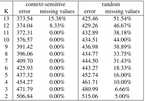
Table 6: Comparison of context-sensitive and random initialization for robust clustering.

context-sensitive random K error missing values error missing values 13 373.54 15.38% 425.46 51.54% 12 374.04 8.33% 429.26 46.67% 11 372.31 0.00% 432.89 38.18% 10 376.57 0.00% 434.51 44.00% 9 391.42 0.00% 436.98 38.89% 8 396.06 0.00% 434.77 33.75% 7 409.70 0.00% 444.50 31.43% 6 425.93 0.00% 443.27 18.33% 5 437.32 0.00% 452.74 16.00% 4 454.27 0.00% 461.71 10.00% 3 471.79 0.00% 480.99 6.66% 2 506.84 0.00% 515.06 5.00%

Dp+1. Thus, throughout the constructive approach full prototypes and small clustering error are favored. The datasetD6, the students who have completed at least half of the core courses, is our actual target data for clustering.

In Table 6, it is shown how the score function changes and the number of missing values with the proposed initialization strategy for different values ofK forD6. For comparison, the table also shows the average results of 10 test runs of the K-spatialmedians algorithm with random initialization. We obtain better results with our approach for the clustering error and, especially, with respect to the missing values. For example, already forK = 3, 6.66% of the prototypes’ values are missing with random initialization and, thus, uninterpretable. Moreover, we also studied the stability of the results by checking whether the students in Dp−1, p ≥ 1, still belong to the same cluster when new students are added and the reclustering ofDp is

performed in Algorithm 2. Confusion matrices between the two consecutive clustering levels were computed. It turned out that the confusion matrices are almost perfect, so that the formation of clusters is very stable and the clusters themselves are reliably structured. We conclude that the proposed context-sensitive initialization provides a clustering result with low error and high interpretability.

Figure 3: Decrease in errors for target data when more clusters are introduced successively.

4.3. ANALYZING THE CLUSTERING RESULTS

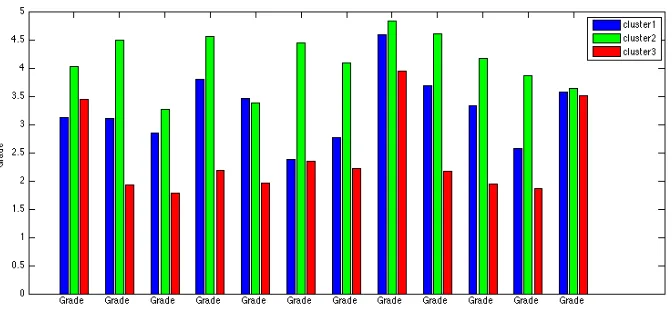
In the first two columns of Table 7, the ranking of the core courses based on their prototype separation is provided. Since the general profile of the three clusters is “medium” (cluster 1), “high” (cluster 2), and “low” (cluster 3), we compute, for each variable, two distances: d1 =

|C2−C1|andd2 =|C3−C1|. The two measures are computed (i) as the mean of{(d1)i,(d2)i}

(denoted asmeasure 1) and (ii) the minimum of{(d1)i,(d2)i}(denoted asmeasure 2). As can

be seen from the table, measures 1 and2 provide practically the same ranking. However, we think that of these two indicators, the second measure provides clearer variable separation. For example, with measure 1 we could have a high distance value for a course even if only one prototype value Ci is very dissimilar from the other two. Moreover, in order to assess even

further the explanative power of variables related to the clustering result withK = 3,we also applied the nonparametric Kruskal-Wallis test (Hollander et al., 2013) to compare the subsets of data in the three clusters. Since the actual clusterwise datasets contain missing values, we used one iteration of thehot deck imputation(Ayr¨am¨o, 2006;¨ Batista and Monard, 2003) to complete them: We imputed the missing values using the cluster prototype values of theK-spatialmedians

Figure 4: Prototypes of the three student clusters.

Table 7: Distances between the clusters.

measure 1 measure 2 Kruskal-Wallis

course code distance rank distance rank χ2 p rank sum (rank) PCtools 0.1472 8 0.3220 8 33.10 ? ? ? 9 17 (9) Datanet 0.8183 1 1.1754 1 84.69 ? ? ? 1 2 (1) OOA&D 0.2249 7 0.4247 7 47.97 ? ? ? 7 14 (6) Alg1 0.6090 3 0.7501 4 82.39 ? ? ? 2 6 (2) IntroSE 0.0588 10 0.0781 10 34 .94 ? ? ? 8 18 (10) OpSys 0.0413 11 0.0402 12 67.06 ? ? ? 4 16 (7) DB&DMgm 0.3666 6 0.5490 6 53.96 ? ? ? 6 12 (5) Prog1 0.0796 9 0.2417 9 32.21 ? ? ? 10 19 (11) Prog2 0.7064 2 0.9309 2 54.35 ? ? ? 5 7 (4) CompArc 0.5872 4 0.8439 3 78.49 ? ? ? 3 6 (3) GUIprog 0.4602 5 0.7118 5 31.04 ? ? ? 11 16 (8) CompRes 0.0021 12 0.0633 11 17.23 ? ? ? 12 23 (12)

Figure 5: Semesterwise credits versus the mean grade in core courses for the students in each cluster.

was expected.

In terms of quality, the students inD6are clearly separated into the three clusters. To check whether the clusters also differentiate the students according to their quantity of studies, we looked also (see Section 2.1 and 3) at the students’ average number of credits. In Figure 5, the semester-wise relation of grades in the core courses and the overall credits of the individual students in the different clusters is visualized. From this figure, we deduce that the students who belong tocluster 2not only are the best when it comes to the average grades in the core courses but also are the most efficient as they earn on average the most number of credits per semester. Likewise, the students in the gradewise low-performingcluster 3also earn the fewest credits per semester (on average eight credits less than the students incluster 2). The correlation coefficient of the mean grade in the core courses and the average number of credits semesterwise per student is0.4415with a p-value that is highly statistically significant. We know that this relation does not exist in the whole student level and when the average of all studies is used (see Figure 1). Thus, we conclude that for the core CS courses, the students who perform well in terms of grades also perform well in terms of the number of courses.

5.

P

popular techniques such as radial basis function networks or support vector machines, which construct their basis in the space of observations. This is an appropriate starting point because our purpose is to assess the importance of the model inputs, which correspond to the core courses being analyzed. In this way, we close our between-method triangulation by contrasting the previous results and conclusions based on unsupervised analysis with the corresponding results from a supervised, predictive technique.

There are many inherent difficulties when a flexible model is used in prediction and trained using a given set of input-output samples. First, because of the universality, such a model could actually represent the discrete dataset precisely (e.g.,Tamura and Tateishi 1997; Huang 2003), which would mean that all the noise in the samples would be reproduced. Thus, one needs to restrict the flexibility of such models. This can be done in two ways: by restricting the size of the network’s configuration (number and size of layers; structural simplicity) or restricting the nonlinearity of the encoded function (size of weights, seeBartlett 1998; functional simplicity). Here we will assess the network’s simplicity along both dimensions, in order to favor and restore the simplest model (cf. Occam’s razor). Second, we look for a prediction model that provides the best generalization of the sample data, and, for this purpose, apply the well-known stratified cross-validation (seeKohavi 1995) to compute an estimate of the generalization error. Stratifi-cation means that, given a certain labeling to encode classes in a discrete dataset, the number of samples in the created folds (subsets) coincides with the sizes of the different classes as closely as possible. Clearly, the number of classes and number of folds do not need to be the same. Third, as in clustering, use of a local optimizer to solve the nonlinear optimization problem to determine the network weights provides only local search (exploitation), and for exploration, we use multiple restarts with random initialization (seeK¨arkk¨ainen 2002). The whole training approach as just summarized has been more thoroughly introduced and tested in K¨arkk¨ainen (2014) and successfully applied in time-series analysis inK¨arkk¨ainen et al.(2014).

Next we will derive and detail the whole predictive approach. First, the MLP neural network and its determination are formalized, and then the overall training algorithm and the input-sensitivity analysis are developed and described.

5.1. PREDICTION WITH INPUT SENSITIVITY ANALYSIS

5.1.1. MLP training approach

The action of the multilayer perceptron in a layered, compact form can be given by (e.g.,Hagan and Menhaj 1994)

o0 =x, ol =Fl_(Wl_˜o(l−1)_{) forl= 1, . . . , L. (3)}

Here the layer number (starting from zero for the input) has been placed as an upper index. By˜ we indicate the addition of bias terms to the transformation, which is realized by enlarging a vec-torvwith constant: v˜T =1 vT

.In practice, this places the bias weights as the first columns of the layer matrices that then have the factorizationWl ₌

Wl 0 Wl1

.Fl_{(·)denotes the}

ap-plication of activation functions on the lth level. Formally, this corresponds to matrix-vector multiplication in which the matrix components are functions, and component multiplication is replaced with application of the corresponding component function (K¨arkk¨ainen, 2002). The di-mensions of the weight-matrices are given bydim(Wl_{) =n}

l×(nl−1+ 1), l= 1, . . . , L,where n0 is the length of an input-vector x, nLthe length of the output-vectoroL,andnl,0< l < L,

Using the given training data {xi,yi}N_i=1, with xi ∈ Rn0 denoting the input-vectors and yi ∈ RnL the output vectors, respectively, the unknown weight matrices {Wl}Ll=1 in (3) are determined as a solution of an optimization problem

min

{Wl_}L l=1

J({Wl}). (4)

We restrict ourselves to MLP with one hidden layer, and the actual cost function reads as follows:

J(W1,W2) = 1 2N

N

X

i=1

N(W1,W2)(x_i)−y_i 2 + β 2n1 X

(i,j)

|W1_i,j|2_+|(W2 1)i,j|

2 (5)

forβ ≥0andN(W1,W2)(xi) = W2F˜1(W1x˜i). The special form of regularization omitting

the bias columnW2

0 is due to Corollary 1 byK¨arkk¨ainen(2002):Every locally optimal solution to (4) with the cost functional (5) provides an unbiased regression estimate having zero mean error over the training data.

The universal approximation property guarantees the potential accuracy of an MLP network for given data and the unbiasedness as just described provides statistical support for its use, but as explained above, we also address the network’s simplicityandgeneralization. Thus, in our actual training method we grid-search the size of the hidden layern1 and the size of the regu-larization coefficientβ: The smallern1, the simpler the structure of the network; and the larger β, the smaller the weight values and the closer the MLP to a (simpler) linear, single-layered network. Moreover, cross-validation is used as the technique to ensure that generalization abil-ity of the network is taken as the main accuracy criterion. Finally, the usual gradient-based optimization methods for minimizing (5) act locally, so that we repeat the optimization with random initialization twice when we search for the values of metaparameters n1 andβ.When they have been fixed, the final network is optimized using five local restarts to further improve the exploration of the search landscape.

The whole training approach for the MLP network is given in Algorithm 3. We use the following set of possible regularization parameter values, which were determined according to prior computational tests:

~

β =10−2 7.5·10−3 5·10−3 2.5·10−3 10−3 7.5·10−4 5·10−4 2.5·10−4 10−4.

The prediction error with a training or test set is computed as the mean Euclidian error

1 N N X i=1

N(W1,W2)(x_i)−y_i

. (6)

We use the most common sigmoidal activation functions s(x) = 1

1+exp(−x) for F

1_{. All input}

variables are preprocessed into the range[0,1]ofs(x)to balance their scaling with each other and with the range of the overall MLP transformation (seeK¨arkk¨ainen 2002for a more thorough argument).

5.1.2. Derivation of input sensitivity of MLP

Algorithm 3:Reliable determination of MLP neural network.

Input: Training data{xi,yi} N i=1.

Output: MLP neural networkN(W1,W2).

Define a vectorβ~of regularization coefficients, maximum size of the hidden layer n1max,andnf olds,the number of folds for cross-validation, created using stratified random sampling;

forn1 ←1ton1maxdo

forregs←1to|β~|(| · |denotes the size of a vector)do fork ←1tonf oldsdo

fori←1to2do

Initialize(W1_,W2_{)from the uniform distributionU([−1,1]);} Minimize (5) with currentn1 andβ(regs),~ and the CV Training set; Store Network for smallest Training Set Prediction Error;

end

Compute Test Set Prediction Error for the stored Network; end

Storen∗₁ =n1 andβ∗ =βfor the smallest mean Test Set Prediction Error; end

end

fori←1to5do

Initialize(W1,W2)fromU([−1,1]);

Minimize (5) usingn∗₁, β∗and the whole training data; end

its input. Seven possible definitions of sensitivity were compared inGevrey et al.(2003) in an ecological context and four of them, further, in relation to chemical engineering inShojaeefard et al. (2013). Both comparisons concluded that in order to assess the relevancy and rank the features, the partial derivatives (PaD) method proposed by Dimopoulos et al.(1995) provides appropriate information and computational coherency in the form of stability. Thus, we also use the analytic partial derivative as the core of the sensitivity measure, but in a more general and more robust fashion thanDimopoulos et al.(1995).

An analytical formula for the MLP input sensitivity can be directly calculated from the layer-wise formula (3). The precise result is stated in the next proposition.

Proposition 1

∇xN({Wl})(x) =

∂oL ∂x =

1

Y

l=L

diag{(Fl₎0_}Wl

1. (7)

HereWl₁ denotes, as before, the lth weight matrix without the first bias column. In particular, for an MLP with one hidden layer and linear output (o2 _=W2_F˜1_(W1_{x˜)), (7) states that}

∂o2 ∂x =W

2

1 diag{(F 1

Algorithm 4:Input sensitivity ranking.

Input: Data(X,Y) = {xi,yi}N_i=1 of inputs and desired outputs.

Output: Ranked list of MLP input variables.

1: Fixβ~ andn1max,and apply Algorithm3to obtainN(W1,W2);

2: Compute MAS ofN(W1,W2)according to formula (9);

3: Order input variables in descending order with respect to MAS to establish ranking;

With the discrete data {xi}Ni=1, input sensitivity must be assessed and computed over the dataset. Thus, we apply (7) to compute the mean absolute sensitivity, MAS (see Ruck et al. 1990):

1 N

N

X

i=1

∂oL ∂xi

(9)

of the trained network for all input variables. After this formula is applied, the approach for input ranking is based on the following concept: The higher the MAS, the more salient the feature is for the network. This is due to the well-known Taylor theorem in calculus related to local approximation of smooth functions (seeApostol 1969). Namely, if a function is locally constant, its gradient vector (i.e., the vector of partial derivatives) is zero, and such a function could be (locally) represented and absorbed to the MLP bias. Thus, the larger the mean sum of the absolute values of the local partial derivatives for an input variable, the more important that input variable is for representing the variability of an unknown function approximated by the MLP. Thus, the descending order of MAS values defines the ranking of input variables over one run of Algorithm 3. The method described by Dimopoulos et al. (1995) starts with the similar analytic formula (formula (3)) as in (7), but (7) is a generalization because our MLP model contains the bias nodes in order to always guarantee unbiased regression estimate for the training data in Algorithm3. Moreover, as with clustering, we compute the overall input-output sensitivity formulae using the robustmean absolute errorinstead of the sum-of-squares proposed in Dimopoulos et al. (1995), which nonuniformly concentrates on large deviations from zero (seeK¨arkk¨ainen and Heikkola 2004).

5.2. PREDICTIVE RESULTS AND THEIR ANALYSIS

As input data for MLP, we use the same set as in the cluster analysis, i.e. the grades of the students who have completed at least half of the core courses; see Table3. Moreover, the miss-ing values (29.65% altogether) are again completed by using the hot-deck imputation with 8 prototypes (see Section 4.3 for more thorough description). As output data, for each student considered, we use (i) the mean grade and (ii) the mean number of credits per semester, individ-ually.

Results of the predictive analysis process, as described above, are provided in Table8. There, for each course, the “RSum” provides the sum of rankings (1–12) of five individual runs of Algorithm4. Moreover, in order to assess the stability of the final ranking, we have tested 3-fold, 7-fold, and 10-fold stratified cross-validation. As labels for the 3-fold stratification, we used the three cluster indices that were obtained in the previous section forK = 3(the analyzed result). For the 7-fold CV, the labels corresponded to the number of completed courses in Table3, i.e., to the separate groups of students forq = 6, . . . ,12, whose sizes are given by nq. In the third

stratified cross-validation strategy with 10 folds, we used the labels that were obtained when clustering the students into8clusters (same as in imputation).

Thus, the strategy to create the different number of stratified folds was completely different, but the final rankings of the 7-fold and 10-fold CV were exactly the same, and there was only one very small difference compared to the 3-fold CV: For the mean grade, rankings of thePCtools and Datanetcourses were swapped. We conclude that there is high reliability concerning the final rankings, because the Fleissκ shows moderate agreementfor grades with 7 and 10 folds and the rest of the cases witnesssubstantial agreementbetween the ratings of the individual runs of Algorithm4. From “MeanError” (see Table8), which represents the mean of the prediction error (6) over the five runs, we conclude that mean grades can be predicted (in the generalization sense as explained above) about twice as accurately as the mean number of credits semesterwise. Again, this illustrates the higher and more random individual variability of the number of credits obtained per semester compared to the level of grades (see also Figures6and7).

Based on the results presented in Table 8, we draw the following main conclusions: Com-pared to the correlation and clustering analysis results, also based on the predictive MLP input sensitivity analysis, the courses Datanetworksand Computer Structure and Architectureseem to be most influential to the overall performance in the studies. For the performance in grades, also the courseObject Oriented Analysis and Design pops up, and, for the overall credits, the largest courseProgramming 2shows (as in the previous analyses) high significance.

For some course, likeComputer and Datanetworks as ToolsandProgramming of Graphical User Interfaces, there is a large difference in the ranks between the mean grades and the mean credits, which was not addressed as strongly by the other two EDM techniques. One reason for this might be the varying number of students passing a course, which is reflected in the predictive analysis as the higher need of imputation. As can be seen from Figure2, many fewer students have passed these two courses compared to the other courses5.

The predictions and the prediction errors for grades and credits, studentwise, are illustrated in Figures6and7. In the figures, the x-axis corresponds to a student index, where the students are taken in the ascending order for missing courses; the larger the index, the more core course grades are missing, and were imputed in the MLP training data. With this respect, the accuracy

Table 8: Input rankings for the three foldings.

3-fold CV 7-fold CV 10-fold CV

grades credits grades credits grades credits MeanError 6.44e-3 1.22e-2 6.37e-3 1.22e-2 6.36e-3 1.22e-2

Fleissκ 0.76 0.72 0.49 0.62 0.52 0.78

Course RSum rank RSum rank RSum rank RSum rank RSum rank RSum rank

PCtools 19 4 49 10 16 3 47 10 15 3 50 10

Datanet 17 3 10 2 19 4 10 2 18 4 10 2

OOA&D 10 2 39 7 12 2 40 7 13 2 39 7

Alg1 30 6 20 4 31 6 20 4 31 6 20 4

IntroSE 36 7 42 9 36 7 42 9 36 7 41 9

OpSys 39 8 57 11 41 8 57 11 41 8 57 11

DB&DMgm 45 9 15 3 42 9 15 3 42 9 15 3

Prog1 60 12 30 6 59 12 32 6 59 12 30 6

Prog2 50 10 5 1 50 10 5 1 50 10 5 1

CompArc 5 1 25 5 6 1 25 5 6 1 25 5

GUIprog 24 5 58 12 22 5 58 12 23 5 58 12

CompRes 55 11 40 8 56 11 41 8 56 11 40 8

of the mean number of credits per semester shows large increase at the end. As can be seen from Figure 6, the grades of the core courses predict, with reasonable accuracy, the overall mean grade level of a student. This result is promising, especially when the number of credits related to the analyzed core courses is typically less than half of the total number of credits; see Table4. In contrast, the generalization accuracy of the average number of credits per semester is very bad (see Figure7), and the last students, i.e., those with the most missing values, are the most erroneous. Thus, we do not recommend the final network for actual prediction, but the network is considered suitable for the sensitivity analysis. The difference between accurate prediction and stable detection of input relevance is also clearly captured in Table8 as explained above: The rankings in the repeated attempts in Table8are very stable, as shown by the Fleissκ’s, even if the prediction accuracy can be very poor as shown in Figures6and7.

Hornik et al.(1989) summarize the essence of MLP training: “We have thus established that such ‘mapping’ networks are universal approximators. This implies that any lack of success in applications must arise from inadequate learning, insufficient numbers of hidden units or the lack of a deterministic relationship between input and target.” The proposed training approach here tries to manage all these issues in order to end up withthe most reliably generalizing MLP network. Thus, we try to capture the deterministic behavior within the data and use this to compute the input relevance. Stability of the results as witnessed in Table 8, with substantial within-method triangulation, supports the conclusion that this was obtained here.

6.

C

Figure 6: Prediction of mean grades: real (green) and predicted (blue) values.

using the available data strategy and prototype-based imputation. In Table9, all analysis results are summarized. We can conclude the study from the educational domain level point of view and from the methodological point of view.

From the domain level point of view and based on Table9, we conclude that the quality of studies is determined by the first introductory courses, Datanetworksand Computer Structure and Architecture, offered in the first year of the program. Both courses test more the general capability of a student to study than the actual knowledge of professional CS skills. Though they have technical topics, they are taught on a conceptual level, and especially compared with the third introductory course (see Table2), they are completed by a final examination at the end of the course. Therefore, these courses test how well the student is able to learn, understand, and explain concepts instead of testing specific (IT) skills. When it comes to credits/timely graduation, a student’s success is also determined by sedulousness and perseverance: The Pro-gramming 2which is also creditwise the largest course (see Table2), is strongly related to the number of credits that a student can earn in general with hard work. Thus, for the overall perfor-mance, general study capabilities are more important than the occupational skills and students can succeed in CS studies with diligent and goal-oriented study behavior without being the most skilled programmers with mathematical talent. This is important knowledge that should be communicated to the students in the beginning of their studies.

Figure 7: Prediction of mean credits: real (green) and predicted (blue) values.

other institutions since educational data and the subsequent knowledge of particular courses are different. From the methodological perspective, however, both overall approach and the individ-ual methods with their varying but argumented details are general and can be applied to analyze the sparse data of student performance. If a snapshot of a study registry of an arbitrary educa-tional institution were taken, there were missing values similarly to our case for the uncompleted courses. And, then, all methods and approaches could be applied. Furthermore, according to our current computational experience, we can conclude that for around a dozen variables (even us-ing Matlab): i) correlation analysis scales up to one million observations, ii) clusterus-ing analysis scales up to hundreds of thousands of observations, and iii) predictive MLP analysis scales up to thousands of observations. This means that our methods can also be used for larger datasets.

construc-Table 9: Summary of the results.

grades credits

course M1 M2 M3 sum (rank) M1 M2 M3 sum (rank) Computer and Datanetworks as Tools 11 9 3 23 (8) 12 9 10 31 (12)

Datanetworks 3 1 4 8 (2) 1 1 2 4 (1)

Object Oriented Analysis and Design 6 6 2 14 (4) 11 6 7 24 (7)

Algorithms 1 1 2 6 9 (3) 4 2 4 10 (3)

Introduction to Software Engineering 10 10 7 27 (10) 9 10 9 28 (10)

Operating Systems 8 7 8 23 (9) 8 7 11 26 (9)

Basics of Databases and Data Management 5 5 9 19 (6) 5 5 3 13 (5)

Programming 1 9 11 12 32 (11) 7 11 6 24 (6)

Programming 2 4 4 10 18 (5) 2 4 1 7 (2)

Computer Structure and Architecture 2 3 1 6 (1) 3 3 5 11 (4) Programming of Graphical User Interfaces 7 8 5 20 (7) 6 8 12 26 (8) Research Methods in Computing 12 12 11 35 (12) 10 12 8 30 (11)

tively initialized and how the variable ranking of prototypes is derived are not standard choices in cluster analysis. Moreover, the whole computational process for the predictive analysis — use of MLP with a) hot-deck imputation, b) complexity-aware training for best generalization, c) analytic formula-based robust input sensitivity derivation, d) sensitivity ranking, e) Fleissκas stability measure for rankings is completely novel. It is also based on our own implementation throughout. Training phase b) has been recently proposed and tested inK¨arkk¨ainen(2014) and K¨arkk¨ainen et al.(2014).

The underlying principle to study soundness in all the treatments here was based on local and global triangulation: In the correlation analysis, significancy was computed with and with-out Bonferroni correction. In cluster analysis, variable ranking was computed in two ways and assessed using the nonparametric Kruskal-Wallis test. Similarly, in the predictive analysis three different foldings (number of folds and how they are created) were used and Fleissκwas then applied to the results of five iterations of the overall algorithm to study its stability. Thus, locally (for each method separately), we have made serious and versatile attempts to vary the meta-parametrization of the approaches and reported all the results. Globally, on the whole analysis level, we have again based our overall conclusions on the results and conclusions of the three methods of different orientations in EDM. We reason that such two-level treatment, where lo-cally and globally the same results and their interpretation are supported by different approaches, improves the technical soundness of the study. Furthermore, the method for obtaining the final ranking, in clustering and in the MLP analysis, is novel and establishes a practical framework that can be used in similar applications.

A

R

ALDAHDOOH, R. T. AND ASHOUR, W. 2013. Dimk-means distance-based initialization method for k-means clustering algorithm. International Journal of Intelligent Systems and Applications (IJISA) 5,2, 41.

APOSTOL, T. M. 1969.Calculus, Volume 2: Multi-variable Calculus and Linear Algebra with Applica-tions to Differential EquaApplica-tions and Probability. Wiley.

¨

AYRAM¨ O¨, S. 2006. Knowledge Mining Using Robust Clustering. Jyv¨askyl¨a Studies in Computing, vol. 63. University of Jyv¨askyl¨a.

BAI, L., LIANG, J.,ANDDANG, C. 2011. An initialization method to simultaneously find initial cluster centers and the number of clusters for clustering categorical data.Knowledge-Based Systems 24,6, 785–795.

BAI, L., LIANG, J., DANG, C.,ANDCAO, F. 2012. A cluster centers initialization method for clustering categorical data.Expert Systems with Applications 39,9, 8022–8029.

BAKER, R. ET AL. 2010. Data mining for education.International Encyclopedia of Education 7, 112– 118.

BAKER, R. S.ANDYACEF, K. 2009. The state of educational data mining in 2009: A review and future

visions.Journal of Educational Data Mining 1,1, 3–17.

BARTLETT, P. L. 1998. The sample complexity of pattern classification with neural networks: the size of the weights is more important than the size of the network.Information Theory, IEEE Transactions on 44,2, 525–536.

BATISTA, G. AND MONARD, M. C. 2003. An analysis of four missing data treatment methods for supervised learning.Applied Artificial Intelligence 17, 519–533.

BAYER, J., BYDZOVSKA´, H., G ´ERYK, J., OBˇSIVAC, T.,ANDPOPELINSKY`, L. 2012. Predicting drop-out from social behaviour of students. InEducational Data Mining 2012. 103–109.

BHARDWAJ, B.ANDPAL, S. 2011. Mining educational data to analyze students’ performance.(IJCSIS) International Journal of Computer Science and Information Security, 9,4.

BOUCHET, F., KINNEBREW, J. S., BISWAS, G., AND AZEVEDO, R. 2012. Identifying students’ char-acteristic learning behaviors in an intelligent tutoring system fostering self-regulated learning. In Educational Data Mining 2012. 65–72.

BRADLEY, P.AND FAYYAD, U. 1998. Refining initial points for k-means clustering. InICML. Vol. 98.

91–99.

BRYMAN, A. 2003. Triangulation.The Sage encyclopedia of social science research methods. Thousand Oaks, CA: Sage.

CALDERS, T. AND PECHENIZKIY, M. 2012. Introduction to the special section on educational data mining.ACM SIGKDD Explorations Newsletter 13,2, 3–6.

CAMPAGNI, R., MERLINI, D., AND SPRUGNOLI, R. 2012. Analyzing paths in a student database. In

Educational Data Mining 2012. 208–209.

CARLSON, R., GENIN, K., RAU, M.,ANDSCHEINES, R. 2013. Student profiling from tutoring system log data: When do multiple graphical representations matter? In Educational Data Mining 2013. 12–20.

CHEN, L., CHEN, L., JIANG, Q., WANG, B.,ANDSHI, L. 2009. An initialization method for clustering high-dimensional data. InDatabase Technology and Applications, 2009 First International Workshop on. IEEE, 444–447.

CROUX, C., DEHON, C.,AND YADINE, A. 2010. Thek-step spatial sign covariance matrix.Adv Data Anal Classif 4, 137–150.

DENZIN, N. 1970. Strategies of multiple triangulation. The research act in sociology: A theoretical introduction to sociological method, 297–313.

DIMOPOULOS, Y., BOURRET, P., AND LEK, S. 1995. Use of some sensitivity criteria for choosing networks with good generalization ability.Neural Processing Letters 2,6, 1–4.

EMRECELEBI, M., KINGRAVI, H. A.,ANDVELA, P. A. 2012. A comparative study of efficient

initial-ization methods for the k-means clustering algorithm.Expert Systems with Applications.

ERDOGAN, S. AND TYMOR, M. 2005. A data mining application in a student database. Journal Of Aeronautics and Space Technologies 2, 53–57.

FAYYAD, U., PIATESKY-SHAPIRO, G., ANDP., S. 1996. Extracting useful knowledge from volumes of data.Communications of the ACM 39,11, pp. 27–34.

FLEISS, J. L. 1971. Measuring nominal scale agreement among many raters. Psychological Bul-letin 76,5, 378–382.

GEVREY, M., DIMOPAULOS, I., AND LEK, S. 2003. Review and comparison of methods to study the contribution of variables in artificial neural network models.Ecological Modelling 160, 249–264.

HAGAN, M. T. AND MENHAJ, M. B. 1994. Training feedforward networks with the Marquardt algo-rithm.IEEE Trans. Neural Networks 5, 989–993.

HALONEN, P. 2012. Tietotekniikan laitos. 2. TIETOTEKNIIKKA 12a- valintasyyt- opetuksen laatu-mielipiteet.pdf.

HAN, J., KAMBER, M.,ANDTUNG, A. 2001. Spatial clustering methods in data mining: A survey.Data Mining and Knowledge Discovery.

HARDEN, T. ANDTERVO, M. 2012. Informaatioteknologian tiedekunta. 1. ITK 4- opinnoista

suoriutu-minen.pdf.

HARPSTEAD, E., MACLELLAN, C. J., KOEDINGER, K. R., ALEVEN, V., DOW, S. P., AND MYERS, B. A. 2013. Investigating the solution space of an open-ended educational game using conceptual feature extraction. InEducational Data Mining 2013. 51–59.

HAWKINS, W., HEFFERNAN, N., WANG, Y.,ANDBAKER, R. S. 2013. Extending the assistance model:

Analyzing the use of assistance over time. InEducational Data Mining 2013. 59–67.

HETTMANSPERGER, T. P. AND MCKEAN, J. W. 1998.Robust nonparametric statistical methods. Ed-ward Arnold, London.

HOLLANDER, M., WOLFE, D. A., AND CHICKEN, E. 2013.Nonparametric statistical methods. Vol. 751. John Wiley & Sons.

HORNIK, K., STINCHCOMBE, M.,ANDWHITE, H. 1989. Multilayer feedforward networks are universal

approximators.Neural Networks 2, 359–366.

HUANG, G. B. 2003. Learning capability and storage capacity of two-hidden-layer feedforward net-works.Neural Networks, IEEE Transactions on 14,2, 274–281.

HUBER, P. J. 1981.Robust Statistics. John Wiley & Sons Inc., New York.

JERKINS, J. A., STENGER, C. L., STOVALL, J., ANDJENKINS, J. T. 2013. Establishing the Impact of a Computer Science/Mathematics Anti-symbiotic Stereotype in CS Students.Journal of Computing Sciences in Colleges 28,5 (May), 47–53.

JICK, T. D. 1979. Mixing qualitative and quantitative methods: Triangulation in action.Administrative science quarterly 24,4, 602–611.

JOHN, G. H., KOHAVI, R.,ANDPFLEGER, K. 1994. Irrelevant features and the subset selection problem. InProceedings of the 11th International Conference on Machine Learning. 121–129.

K ¨ARKKAINEN¨ , T. 2002. MLP in layer-wise form with applications in weight decay.Neural Computa-tion 14, 1451–1480.

K ¨ARKKAINEN¨ , T. 2014. Feedforward Network - With or Without an Adaptive Hidden Layer. IEEE

Transactions on Neural Networks and Learning Systems. In revision.

K ¨ARKKAINEN¨ , T. ANDA¨YRAM¨ O¨, S. 2005. On computation of spatial median for robust data mining. Evolutionary and Deterministic Methods for Design, Optimization and Control with Applications to Industrial and Societal Problems, EUROGEN, Munich.

K ¨ARKKAINEN¨ , T. ANDHEIKKOLA, E. 2004. Robust formulations for training multilayer perceptrons.

Neural Computation 16, 837–862.

K ¨ARKKAINEN¨ , T., MASLOV, A.,ANDWARTIAINEN, P. 2014. Region of interest detection using MLP. In Proceedings of the European Symposium on Artificial Neural Networks, Computational Intelli-gence and Machine Learning - ESANN 2014. 213–218.

K ¨ARKKAINEN¨ , T. AND TOIVANEN, J. 2001. Building blocks for odd–even multigrid with applications

to reduced systems.Journal of computational and applied mathematics 131,1, 15–33.

KERR, D.AND CHUNG, G. 2012. Identifying key features of student performance in educational video games and simulations through cluster analysis.Journal of Educational Data Mining 4,1, 144–182.

KHAN, S. S. AND AHMAD, A. 2013. Cluster center initialization algorithm for k-modes clustering. Expert Systems with Applications.

KINNUNEN, P., MARTTILA-KONTIO, M.,ANDPESONEN, E. 2013. Getting to know computer science freshmen. InProceedings of the 13th Koli Calling International Conference on Computing Education Research. Koli Calling ’13. ACM, New York, NY, USA, 59–66.

KOHAVI, R. 1995. Study of cross-validation and bootstrap for accuracy estimation and model selection. In Proceedings of the International Joint Conference on Artificial Intelligence (IJCAI’95). 1137– 1143.

KOHAVI, R. AND JOHN, G. H. 1997. Wrappers for feature subset selection.Artificial Intelligence 97, 273–324.

KOTSIANTIS, S. 2012. Use of machine learning techniques for educational proposes: a decision support

system for forecasting students grades.Artificial Intelligence Review 37,4, 331–344.

MEILA˘, M. AND HECKERMAN, D. 1998. An experimental comparison of several clustering and ini-tialization methods. InProceedings of the 14th Conference on Uncertainty in Artificial Intelligence. Morgan Kaufmann Publishers Inc., 386–395.

MENDEZ, G., BUSKIRK, T., LOHR, S., AND HAAG, S. 2008. Factors associated with persistence in

science and engineering majors: An exploratory study using classification trees and random forests. Journal of Engineering Education 97,1.

RICE, W. R. 1989. Analyzing tables of statistical tests.Evolution 43,1, 223–225.

ROUSSEEUW, P. J. AND LEROY, A. M. 1987. Robust regression and outlier detection. John Wiley & Sons Inc., New York.

RUBIN, D. B. 1976. Inference and missing data.Biometrika 63,3, 581–592.

RUBIN, D. B.ANDLITTLE, R. J. 2002. Statistical analysis with missing data.Hoboken, NJ: J Wiley & Sons.

RUCK, D. W., ROGERS, S. K.,ANDKABRISKY, M. 1990. Feature selection using a multilayer

percep-tron.Neural Network Computing 2,2, 40–48.

SAARELA, M. AND K ¨ARKKAINEN¨ , T. 2014. Discovering Gender-Specific Knowledge from Finnish Basic Education using PISA Scale Indices. InEducational Data Mining 2014. 60–68.

SAHAMI, M., DANYLUK, A., FINCHER, S., FISHER, K., GROSSMAN, D., HAWTHRONE, E., KATZ, R., LEBLANC, R., REED, D., ROACH, S., CUADROS-VARGAS, E., DODGE, R., KUMAR, A.,

ROBINSON, B., SEKER, R.,ANDTHOMPSON, A. 2013a. Computer science curricula 2013.

SAHAMI, M., ROACH, S., CUADROS-VARGAS, E.,AND LEBLANC, R. 2013b. ACM/IEEE-CS Com-puter Science Curriculum 2013: Reviewing the Ironman Report. In Proceeding of the 44th ACM Technical Symposium on Computer Science Education. ACM, New York, USA, 13–14.

SAN PEDRO, M. O. Z., BAKER, R. S., BOWERS, A. J., AND HEFFERNAN, N. T. 2013. Predicting

college enrollment from student interaction with an intelligent tutoring system in middle school. In Educational Data Mining 2013. 177–184.

SHOJAEEFARD, M. H., AKBARI, M., TAHANI, M., AND FARHANI, F. 2013. Sensitivity analysis of the artificial neural network outputs in friction stir lap joining of aluminum to brass. Advances in Material Science and Engineering 2013, 1–7.

SPRINGER, A., JOHNSON, M., EAGLE, M.,ANDBARNES, T. 2013. Using sequential pattern mining to increase graph comprehension in intelligent tutoring system student data. InProceeding of the 44th ACM technical symposium on Computer science education. ACM, 732–732.

STEINBACH, M., ERTOZ¨ , L., AND KUMAR, V. 2004. The challenges of clustering high dimensional data. InNew Directions in Statistical Physics. Springer, 273–309.

TAMURA, S.ANDTATEISHI, M. 1997. Capabilities of a four-layered feedforward neural network: Four layers versus three.IEEE Transactions on Neural Networks 8,2, 251–255.

VALSAMIDIS, S., KONTOGIANNIS, S., KAZANIDIS, I., THEODOSIOU, T.,ANDKARAKOS, A. 2012. A

clustering methodology of web log data for learning management systems.Educational Technology & Society 15,2, 154–167.

VIHAVAINEN, A., LUUKKAINEN, M.,ANDKURHILA, J. 2013. Using students’ programming behavior to predict success in an introductory mathematics course. InEducational Data Mining 2013. 300– 303.

XU, R. AND WUNSCH, D. C. 2005. Survey of clustering algorithms. IEEE Transactions on Neural Networks 16,3, 645–678.