Samira EL YACOUBI, Larbi AFIFI, El Hassan ZERRIK, Abdessamad TRIDANE, Editors
TOWARDS A NEW VIEWPOINT ON
CAUSALITY FOR TIME SERIES
M. FLIESS
1,2and C. JOIN
3 2,4En hommage amical au Professeur Abdelhaq EL JAI
Abstract. Causation between time series is a most important topic in econometrics, financial engi-neering, biological and psychological sciences, and many other fields. A new setting is introduced for examining this rather abstract concept. The corresponding calculations, which are much easier than those required by the celebrated Granger-causality, do not necessitate any deterministic or probabilistic modeling. Some convincing computer simulations are presented.
R´esum´e. La causalit´e entre chroniques est un sujet capital en ´econom´etrie, ing´enierie financi`ere, sciences biologiques et psychologiques, et quantit´e d’autres domaines. On introduit ici une nouvelle approche pour traiter ce concept abstrait. Les calculs, qui sont beaucoup plus simples que ceux li´es `a la causalit´e de Granger, bien connue, ne n´ecessitent aucune mod´elisation, d´eterministe ou probabiliste. On pr´esente plusieurs simulations num´eriques r´eussies.
1.
Introduction
1.1.
Generalities
Causality, or thetheory of causation, is since ever a philosophical mainstay. This is shown by a huge body of writings due to important thinkers like Aristotle, Hume, Kant, Maine de Biran, Mach, Schlick, Meyerson, Carnap, and many others. Let us nevertheless illustrate the difficulty of this concept via the following humorous citation from Bertrand Russell [39]:
The law of causality, I believe, like much that passes muster among philosophers, is a relic of a bygone age, surviving, like the monarchy, only because it is erroneously supposed to do no harm.
1.2.
Granger-causality
More recently causality has been investigated via probabilistic tools (see, e.g., Reichenbach [37], Suppes [43], Pearl [36], . . . ). This is also the case of the Granger-causality [23–25] on time series, to which the names of
1 LIX (CNRS, UMR 7161), ´Ecole polytechnique, 91128 Palaiseau, France.
2 AL.I.E.N. (ALg`ebre pour Identification & Estimation Num´eriques),
24-30 rue Lionnois, BP 60120, 54003 Nancy, France. 3 CRAN (CNRS, UMR 7039), Universit´e de Lorraine,
BP 239, 54506 Vandœuvre-l`es-Nancy, France. 4 Projet Non-A, INRIA Lille – Nord-Europe, France.
c
EDP Sciences, SMAI 2015
Wiener [44] and Sims [40] are often associated. It has gained a huge popularity which is largely due to the following facts:
• Granger-causality is easy and pragmatic, i.e., it seems to bypass to a large extent any philosophical debate.
• Time is naturally incorporated.
Those attractive features lead to the attribution of the Nobel Prize in economic sciences to Granger in 2003 [26].1 A time seriesY is said there to be a “cause” of a time seriesX if, and only if, the forecast ofXbenefits from the knowledge of the past of Y. Granger-causality, which was introduced for answering questions stemming from econometrics and financial engineering and was further developed in many other domains, like, for instance, biology and psychology, has unfortunately not been as successful as many researchers and practitioners hoped. The explanation lies perhaps in its most severe mathematical assumptions, on the
• linear structure of the time series,
• covariance stationarity of the corresponding signals.
They can be only partly weakened via complex operations like cointegration (see, e.g., [6,26,27]). In spite of several attempts to obtain a nonlinear extension, no theory has been adopted and applied on a large scale to the best of our knowledge.
Remark 1. See [35] for a well written historical account of the classic approach to time series in econometrics, where Granger’s works play a key rˆole.
1.3.
Our approach
This paper suggests a quite different route for examining causality between time series. A theorem by Cartier and Perrin [3] is fundamental. It was already presented in [12] where the connection with financial engineering was developed (see also [13,15–17]). Let us summarize some important features of this new standpoint:
(1) The existence oftrends.2
(2) The existence ofquick fluctuations, which yield another setting for classic quantities like volatility [16]. (3) There is no need of a mathematical modeling of the time series. According to our opinion this need
might be the key explanation of the difficulties encountered today by the theory of time series.3 Uncertainty is then taken into account without the need any probabilistic law. We utilize the definition ofbeta
(β) in [15], where some shortcomings of the classic market, or systematic, risk were examined. Introduce for two given time series X,Y theiraveraged means AV∆X, AV∆Y during a time interval ∆. The quotient
βYX(∆, t) =AV∆X AV∆Y
or more precisely, its variation, defines therelation, orinfluence,4betweenX andY at timet. In plain words, the series X and Y are said to be, or not to be, related if the corresponding values of β may be related as follows :
• If |β| isappreciable,5 i.e., is neither too small nor too big, and if β has a constant sign during a quite “long” timeT, we say that one series ispositively(resp. negatively)relatedto the other during the time lapse T ifβ >0 (resp. β <0).
• If the sign ofβ is changing too often, we say that there is no relation between the series.
1Sims also got in 2011 the Nobel prize. Its Nobel lecture on modeling [41] will be discussed elsewhere. See, nevertheless, [12,17],
[14], and Section1.3.
2This is a key assumption intechnical analysisorcharting(see,e.g., [1,32] and the references therein). The notion of trends in
the usual time series literature (see,e.g., [22,30]) does no coincide with ours.
3See [14] for amodel-freecontrol setting, which is most successful from an applied viewpoint.
It might be interesting to
• introduce a different time intervals on the mean averages in order to take into account delays, • give a more canonical value toβ by computing it viareturns.
The forecast ofβthanks to techniques which started in [12] yields moreover a prediction of the relation between the series.
Remark 2. As already stated in [12,13,15–17], our approach is connected to recent advances in control engineering and in signal processing.6 Let us point out therefore that previous works in control have already been employed to analyze some aspects of the theory of causation:
(1) When the differential equations governing a system are known, the control variables, i.e., the causes may be deduced [7].
(2) Determinismin discrete-time may be confirmed in the same way as for deterministic ordinary differential equations in continuous time [8,9].
1.4.
Organization of the paper
Our paper is organized as follows. Section 2 summarizes our viewpoint on time series, which has already been expounded elsewhere (see, e.g., [12,17]). Section3 extracts from [15] the necessary material on the new coefficientβ. The academic time series for the numerical experiments displayed in Section4, which are borrowed from [29], are, as in [28,29],7given by closed-form continuous-time expressions. Some short concluding remarks may be found in Section 5.
2.
Time series
2.1.
Nonstandard analysis and the Cartier-Perrin theorem
8Take the time interval [0,1]⊂Rand introduce as often innonstandard analysis the infinitesimal sampling
T={0 =t0< t1<· · ·< tN = 1}
wheretι+1−tι, 0≤ι < N, isinfinitesimal,i.e., “very small”.9 Atime series X(t) is a functionX :T→R. The Lebesgue measure on T is the function ` defined on T\{1} by `(ti) = ti+1−ti. The measure of any
interval [c, d]⊂T,c≤d, is its lengthd−c. Theintegral over [c, d] of the time seriesX(t) is the sum
Z
[c,d]
Xdτ = X
t∈[c,d]
X(t)`(t)
X is said to be S-integrableif, and only if, for any interval [c, d] the integral R[c,d]|X|dτ is limited, i.e., not infinitely large, and, ifd−cis infinitesimal, also infinitesimal.
X isS-continuousattι∈Tif, and only if,f(tι)'f(τ) whentι 'τ.10 X is said to bealmost continuousif,
and only if, it isS-continuous onT\R, whereR is araresubset.11 X is Lebesgue integrableif, and only if, it isS-integrable and almost continuous.
6The connection between time series and control has been investigated quite a lot in the literature (see,e.g., [2]).
7Note that those two references [28,29] are studying Granger-causality for a better understanding of some questions stemming
from neurosciences.
8See [12] for a more thorough introduction on this theorem, and on nonstandard analysis. Many more citations are also given. 9See,e.g., [4,5] for basics in nonstandard analysis.
10a'bmeans thata−bis infinitesimal.
A time seriesX :T→Ris said to bequickly fluctuating, oroscillating, if, and only if, it isS-integrable and
R
AXdτ is infinitesimal for anyquadrablesubset. 12
Let X : T → R be a S-integrable time series. Then, according to the Cartier-Perrin theorem [3],13 the additive decomposition
X(t) =E(X)(t) +Xfluctuat(t) (1)
holds where
• themean E(X)(t) is Lebesgue integrable, • Xfluctuat(t) is quickly fluctuating.
The decomposition (1) is unique up to an additive infinitesimal quantity.
Remark 3. The notion of quick fluctuations has been employed since [10] as a new approach to noise in automatic control and signal processing. Let us emphasize that this setting was successfully utilized for obtaining powerful estimation and identification techniques (see,e.g., [18–21,42], and the references therein). See [11] for another advances in signal processing, which are based on nonstandard analysis.
2.2.
Variances and covariances
2.2.1. Squares and products
Take twoS-integrable time seriesX(t),Y(t), such that their squares and the squares ofE(X)(t) andE(Y)(t) are alsoS-integrable. The Cauchy-Schwarz inequality shows that the products
• X(t)Y(t),E(X)(t)E(Y)(t),
• E(X)(t)Yfluctuation(t),Xfluctuation(t)E(Y)(t),
• Xfluctuation(t)Yfluctuation(t)
are allS-integrable.
2.2.2. Differentiability
Assume moreover thatE(X)(t) andE(Y)(t) aredifferentiablein the following sense: there exist two Lebesgue integrable time seriesf, g:T→R, such that, for anyt∈T, with the possible exception of a limited number of values oft, E(X)(t) =E(X)(0) +Rt
0f(τ)dτ,E(Y)(t) =E(Y)(0) + Rt
0g(τ)dτ. Integrating by parts shows that
the productsE(X)(t)Yfluctuation(t) andXfluctuation(t)E(Y)(t) are quickly fluctuating [10].
Remark 4. Let us emphasize that the product
Xfluctuation(t)Yfluctuation(t)
is not necessarily quickly fluctuating. This most easily verified by settingXfluctuation(t) =±1, andYfluctuation(t) =
Xfluctuation(t). Then
Xfluctuation(t)Yfluctuation(t) = (Xfluctuation(t)) 2
= 1
2.2.3. Definitions
(1) Thecovariance of two time seriesX(t) andY(t) is
cov(XY)(t) = E((X−E(X))(Y −E(Y))) (t) ' E(XY)(t)−E(X)(t)×E(Y)(t)
12A set isquadrable [3] if its boundary is rare.
(2) Thevariance of the time seriesX(t) is
var(X)(t) = E (X−E(X))2
(t)
' E(X2)(t)−(E(X)(t))2
(3) Thevolatility ofX(t) is the corresponding standard deviation
vol(X)(t) =pvar(X)(t) (2)
The volatility of a quite arbitrary time series seems to be precisely defined here for the first time.
2.3.
Returns
2.3.1. Definition
Assume from now on that, for anyt∈T,
0< m < X(t)< M
wherem,M areappreciable.
Remark 5. This is a realistic assumption ifX(t) is the price of some financial asset. IfX(t) is a temperature, express it in Kelvin degrees, for instance.
The logarithmic return, or log-return, of X with respect to some limited time interval ∆T >0 is the time seriesR∆T defined by
R∆T(X)(t) = ln
X(t)
X(t−∆T)
= lnX(t)−lnX(t−∆T)
From X(Xt−(t∆)T)= 1 + X(tX)−(tX−(∆t−T∆)T), we know that
R∆T(X)(t)'
X(t)−X(t−∆T)
X(t−∆T) (3)
ifX(t)−X(t−∆T) is infinitesimal. The right handside of Equation (3) is thearithmeticreturn. Thenormalized logarithmic return is
r∆T(X)(t) =
R∆T(t)
∆T (4)
2.3.2. Mean
ReplaceX :T→Rby
lnX :T→R, t7→ln (X(t))
where the logarithms of the prices are taken into account. Apply the Cartier-Perrin theorem to lnX. Themean, oraverage, ofr∆T(t) given by Equation (4) is
¯
r∆T(X)(t) =
E(lnX)(t)−E(lnX)(t−∆T)
∆T (5)
As a matter of factr∆T(X) and ¯r∆T(X) are related by
Assume thatE(X) andE(lnX) are differentiable according to Section2.2.2. Call the derivative ofE(lnX) the
normalized mean logarithmic instantaneous returnand write
¯
r(X)(t) = d
dtE(lnX)(t) (6)
Note thatE(lnX)(t)'ln (E(X)(t)) if in Equation (1)Xfluctuation(t)'0. Then ¯r(X)(t)'
d dtE(X)(t)
E(X)(t) .
2.3.3. Volatility
Formulae (2), (4), (5), (6) yield the following mathematical definition of thevolatility of the time seriesX when computed via its retun:
vol∆T(X)(t) = p
E(r∆T −r¯∆T)2(t) (7)
It yields
vol∆T(X)(t)' q
E(r2
∆T)(t)−(¯r∆T(t))2
3.
Beta
It is well known that the coefficient β was introduced in financial engineering for studying some types of
risks. The presentation below is inspired by [15].
3.1.
Arithmetical average
Assume that X :T→R isS-integrable. Take a quadrable set A ⊆T such thatR
Adτ is appreciable. The arithmetical average ofX onA, which is written AVA(X), is defined by
AVA(X) = R
AXdτ R
Adτ
It follows at once from Equation (1) that the difference between AVA(X) and AVA(E(X)) is infinitesimal,i.e.,
AVA(X)'AVA(E(X))
In practice,A is a time interval [t−L, t], with an appreciable lengthL. Set, ift≥L,
X(L, t) = AV[t−L,t](X) = Rt
t−LXdτ
L '
Rt
t−LE(X)dτ
L
3.2.
A formula for betas
Take two
• S-integrable time series X, Y :T→R, • quantitiesLX, LY >0.
Ift >sup(LX, LY) and ifY(LY, t) is appreciable, set
βX,LX
Y,LY (t) =
X(LX, t)
IfLX =LY =L, set
βYX(L, t) =βY,LX,L(t) =X(L, t)
Y(L, t) (8)
Therelation, orinfluence, between X and Y has been already defined in Section1.3. It depends of course on the numerical values ofβX
Y (L, t).
4.
Numerical experiments
The academic time series, who are extracted from [29], i.e., a paper on neurosciences, are given by closed form expressions. There is no room here for studying data from real life.
Remark 6. All the βs in this Section are computed by taking the returns of the time series.
4.1.
Case 1
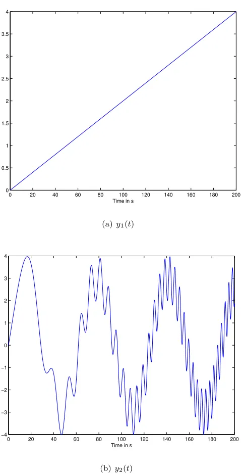
Figure1 displays the two time series
(
y1(t) = 50t
y2(t) = sin( t
2
200) + 3 sin( t 10)
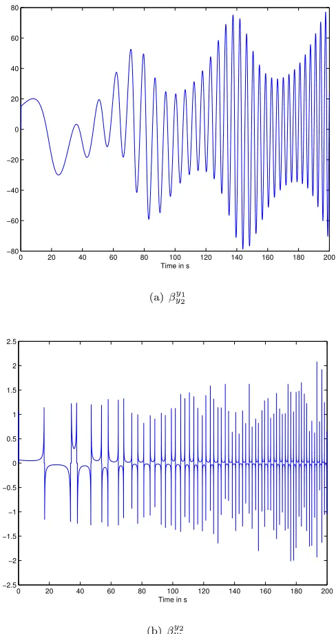
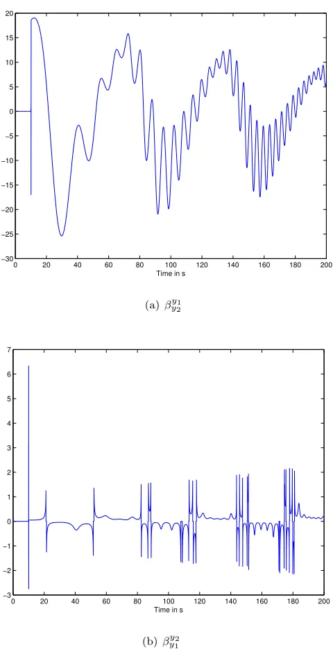
As shown by Figure2there is no clear-cut relation after some time,i.e.,t'80, with a short time lapseL= 0.1 in Equation (8). This is explained of course by the term sin(200t2 ). If the time lapse L becomes larger, i.e., L= 10s, a relation may be read on Figure 3, since the influence of sin(200t2 ) is reduced.
4.2.
Case 2
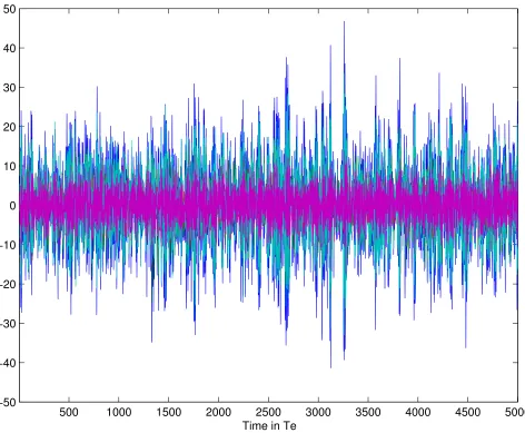
The five time series in Figure4are borrowed from [29]:
x1(t) = .95
√
2x1(t−1)−0.9025x1(t−2) +1(t)
+a16(t) +b17(t) +c17(t−2)
x2(t) = .5x1(t−2) +2(t) +a26(t) +b27(t−1) +c27(t−2)
x3(t) = −.4x1(t−3) +3(t) +a36(t) +b37(t−1) +c37(t−2)
x4(t) = −.5x1(t−2) +.25
√
2x4(t−1) +.25
√
2x5(t−1) +4(t)
+a46(t) +b47(t−1) +c47(t−2)
x5(t) = −.25
√
2x4(t−1) +.25
√
2x5(t−1) +5(t)
+a56(t) +b57(t−1) +c57(t−2)
(9)
where
• i(t),i= 1,· · ·,7, are zero-mean uncorrelated processes with identical variances;
• the coefficients ai, which represent exogenous inputs, are randomly chosen between 0 and 1;
• the terms bi7(t−1) +ci7(t−2), bi = 2, ci = 5, i = 1,2,· · ·,7, represent the influence of latent
variables.
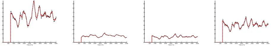
Figure5 displays the variousβji,i, j= 1, . . . ,7,i6=j, with a window length equal to 200Te, whereTeis the
0 20 40 60 80 100 120 140 160 180 200 0
0.5 1 1.5 2 2.5 3 3.5 4
Time in s
(a)y1(t)
0 20 40 60 80 100 120 140 160 180 200
−4 −3 −2 −1 0 1 2 3 4
Time in s
(b)y2(t)
Figure 1. Time evolution of signals
5.
Conclusion
Let us stress again that this new setting for causality between time series, which has been outlined here, does not need any complex deterministic or probabilistic mathematical modeling.14 It seems moreover to be rather straightforward to implement. Its interest, which is obviously connected to some questions about big data, will be hopefully soon confirmed via concrete case-studies, like, for instance, meteorology, where our approach to time series begins to be employed [31].
0 20 40 60 80 100 120 140 160 180 200 −80
−60 −40 −20 0 20 40 60 80
Time in s
(a)βy1
y2
0 20 40 60 80 100 120 140 160 180 200 −2.5
−2 −1.5 −1 −0.5 0 0.5 1 1.5 2 2.5
Time in s
(b)βy2
y1
Figure 2. Betas computed on a short time intervalL= 0.1s
References
[1] T. B´echu, E. Bertrand, J. Nebenzahl,L’analyse technique(6e´ed.). Economica, 2008.
[2] G.E.P. Box, G.M. Jenkins, G.C. Reinsel,Time Series Analysis: Forecasting, and Control(4thed.). Wiley, 2011.
[3] P. Cartier, Y. Perrin, Integration over finite sets. F. & M. Diener (Eds): Nonstandard Analysis in Practice. Springer, 1995, 195–204.
[4] F. Diener, M. Diener,Tutorial. F. & M. Diener (Eds): Nonstandard Analysis in Practice. Springer, 1995, 1–21. [5] F. Diener, G. Reeb,Analyse non standard. Hermann, 1989.
0 20 40 60 80 100 120 140 160 180 200 −30
−25 −20 −15 −10 −5 0 5 10 15 20
Time in s
(a)βy1
y2
0 20 40 60 80 100 120 140 160 180 200 −3
−2 −1 0 1 2 3 4 5 6 7
Time in s
(b)βy2
y1
Figure 3. Betas computed on a long time intervalL= 10s
[7] M. Fliess, Automatique, alg`ebre diff´erentielle et causalit´e. In M. Lothaire (Ed.): M´elanges offerts `a M.-P. Sch¨utzenberger, Herm`es, 1990, 328–334.
[8] M. Fliess, Reversible linear and nonlinear discrete-time dynamics.IEEE Trans. Automat. Control,37, 1992,1144–1153. [9] M. Fliess, Invertibility of causal discrete time dynamical systems.J. Pure Appl. Algebra,86, 1993, 173–179
[10] M. Fliess, Analyse non standard du bruit. C.R. Acad. Sci. Paris Ser. I, 342, 2006, 797–802. Available at http://hal.archives-ouvertes.fr/inria-00001134/en/
500 1000 1500 2000 2500 3000 3500 4000 4500 5000 −50
−40 −30 −20 −10 0 10 20 30 40 50
Time in Te
Figure 4. Time evolution ofxi,i= 1,2,· · · ,7
[12] M. Fliess, C. Join, A mathematical proof of the existence of trends in financial time series. In A. El Jai, L. Afifi, E. Zerrik (Eds): Systems Theory: Modeling, Analysis and Control, Presses Univ. Perpignan, 2009, 43–62. Available at
http://hal.archives-ouvertes.fr/inria-00352834/en/
[13] M. Fliess, C. Join, Preliminary remarks on option pricing and dynamic hedging. 1st Internat. Conf. Syst. Comput. Sci., Villeneuve-d’Ascq, 2012. Available at
http://hal.archives-ouvertes.fr/hal-00705373/en/
[14] M. Fliess, C. Join, Model-free control.Int. J. Control,86, 2013, 2228–2252. Available at
http://hal.archives-ouvertes.fr/hal-00828135/en/
[15] M. Fliess, C. Join, Systematic and multifactor risk models revisited.1st Paris Financial Management Conf., Paris, 2013. Available at
500 1000 1500 2000 2500 3000 3500 4000 4500 5000 −20 −10 0 10 20 30
Time in Te
(a)βx2
x1
500 1000 1500 2000 2500 3000 3500 4000 4500 5000 −20 −10 0 10 20 30
Time in Te
(b)βx3
x1
500 1000 1500 2000 2500 3000 3500 4000 4500 5000 −20 −10 0 10 20 30
Time in Te
(c)βx4
x1
500 1000 1500 2000 2500 3000 3500 4000 4500 5000 −20 −10 0 10 20 30
Time in Te
(d)βx5
x1
500 1000 1500 2000 2500 3000 3500 4000 4500 5000 −20 −10 0 10 20 30
Time in Te
(e)βx1
x2
500 1000 1500 2000 2500 3000 3500 4000 4500 5000 −20 −10 0 10 20 30
Time in Te
(f)βx3
x2
500 1000 1500 2000 2500 3000 3500 4000 4500 5000 −20 −10 0 10 20 30
Time in Te
(g)βx4
x2
500 1000 1500 2000 2500 3000 3500 4000 4500 5000 −20 −10 0 10 20 30
Time in Te
(h)βx5
x2
500 1000 1500 2000 2500 3000 3500 4000 4500 5000 −20 −10 0 10 20 30
Time in Te
(i) βx1
x3
500 1000 1500 2000 2500 3000 3500 4000 4500 5000 −20 −10 0 10 20 30
Time in Te
(j)βx2
x3
500 1000 1500 2000 2500 3000 3500 4000 4500 5000 −20 −10 0 10 20 30
Time in Te
(k)βx4
x3
500 1000 1500 2000 2500 3000 3500 4000 4500 5000 −20 −10 0 10 20 30
Time in Te
(l)βx5
x3
500 1000 1500 2000 2500 3000 3500 4000 4500 5000 −20 −10 0 10 20 30
Time in Te
(m)βx1
x4
500 1000 1500 2000 2500 3000 3500 4000 4500 5000 −20 −10 0 10 20 30
Time in Te
(n)βx2
x4
500 1000 1500 2000 2500 3000 3500 4000 4500 5000 −20 −10 0 10 20 30
Time in Te
(o)βx3
x4
500 1000 1500 2000 2500 3000 3500 4000 4500 5000 −20 −10 0 10 20 30
Time in Te
(p)βx4
x4
500 1000 1500 2000 2500 3000 3500 4000 4500 5000 −20 −10 0 10 20 30
Time in Te
(q)βx1
x5
500 1000 1500 2000 2500 3000 3500 4000 4500 5000 −20 −10 0 10 20 30
Time in Te
(r)βx2
x5
500 1000 1500 2000 2500 3000 3500 4000 4500 5000 −20 −10 0 10 20 30
Time in Te
(s)βx3
x5
500 1000 1500 2000 2500 3000 3500 4000 4500 5000 −20 −10 0 10 20 30
Time in Te
(t)βx4
x5
500 1000 1500 2000 2500 3000 3500 4000 4500 5000 0 1 2 3 4 5 6 7 8 9
Time in Te
(a) Trend of βx2
x1 (red−) and
25T eforecast (black−−)
500 1000 1500 2000 2500 3000 3500 4000 4500 5000 0 1 2 3 4 5 6 7 8 9
Time in Te
(b) Trend ofβx3
x1 (red −) and
25T eforecast (black−−)
500 1000 1500 2000 2500 3000 3500 4000 4500 5000 0 1 2 3 4 5 6 7 8 9
Time in Te
(c) Trend of βx4
x1 (red −) and
25T eforecast (black−−)
500 1000 1500 2000 2500 3000 3500 4000 4500 5000 0 1 2 3 4 5 6 7 8 9
Time in Te
(d) Trend ofβx5
x1 (red −) and
25T eforecast (black−−)
500 1000 1500 2000 2500 3000 3500 4000 4500 5000 0 1 2 3 4 5 6 7 8 9
Time in Te
(e) Trend of βx1
x2 (red−) and
25T eforecast (black−−)
500 1000 1500 2000 2500 3000 3500 4000 4500 5000 0 1 2 3 4 5 6 7 8 9
Time in Te
(f) Trend of βx3
x2 (red −) and
25T eforecast (black−−)
500 1000 1500 2000 2500 3000 3500 4000 4500 5000 0 1 2 3 4 5 6 7 8 9
Time in Te
(g) Trend of βx4
x2 (red−) and
25T eforecast (black−−)
500 1000 1500 2000 2500 3000 3500 4000 4500 5000 0 1 2 3 4 5 6 7 8 9
Time in Te
(h) Trend ofβx5
x2 (red −) and
25T eforecast (black−−)
500 1000 1500 2000 2500 3000 3500 4000 4500 5000 0 1 2 3 4 5 6 7 8 9
Time in Te
(i) Trend of βx1
x3 (red −) and
25T eforecast (black−−)
500 1000 1500 2000 2500 3000 3500 4000 4500 5000 0 1 2 3 4 5 6 7 8 9
Time in Te
(j) Trend of βx2
x3 (red −) and
25T eforecast (black−−)
500 1000 1500 2000 2500 3000 3500 4000 4500 5000 0 1 2 3 4 5 6 7 8 9
Time in Te
(k) Trend of βx4
x3 (red−) and
25T eforecast (black−−)
500 1000 1500 2000 2500 3000 3500 4000 4500 5000 0 1 2 3 4 5 6 7 8 9
Time in Te
(l) Trend of βx5
x3 (red −) and
25T eforecast (black−−)
500 1000 1500 2000 2500 3000 3500 4000 4500 5000 0 1 2 3 4 5 6 7 8 9
Time in Te
(m) Trend of βx1
x4 (red−) and
25T eforecast (black−−)
500 1000 1500 2000 2500 3000 3500 4000 4500 5000 0 1 2 3 4 5 6 7 8 9
Time in Te
(n) Trend ofβx2
x4 (red −) and
25T eforecast (black−−)
500 1000 1500 2000 2500 3000 3500 4000 4500 5000 0 1 2 3 4 5 6 7 8 9
Time in Te
(o) Trend of βx3
x4 (red−) and
25T eforecast (black−−)
500 1000 1500 2000 2500 3000 3500 4000 4500 5000 0 1 2 3 4 5 6 7 8 9
Time in Te
(p) Trend ofβx4
x4 (red −) and
25T eforecast (black−−)
500 1000 1500 2000 2500 3000 3500 4000 4500 5000 0 1 2 3 4 5 6 7 8 9
Time in Te
(q) Trend of βx1
x5 (red −) and
25T eforecast (black−−)
500 1000 1500 2000 2500 3000 3500 4000 4500 5000 0 1 2 3 4 5 6 7 8 9
Time in Te
(r) Trend of βx2
x5 (red −) and
25T eforecast (black−−)
500 1000 1500 2000 2500 3000 3500 4000 4500 5000 0 1 2 3 4 5 6 7 8 9
Time in Te
(s) Trend of βx3
x5 (red −) and
25T eforecast (black−−)
500 1000 1500 2000 2500 3000 3500 4000 4500 5000 0 1 2 3 4 5 6 7 8 9
Time in Te
(t) Trend of βx4
x5 (red −) and
25T eforecast (black−−)
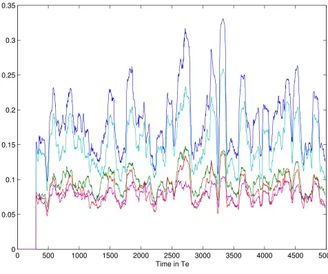
0 500 1000 1500 2000 2500 3000 3500 4000 4500 5000 0
0.05 0.1 0.15 0.2 0.25 0.3 0.35
Time in Te
Figure 7. Time evolution ofvol10T e(xi)(t),i= 1,2,· · · ,7
[16] M. Fliess, C. Join, F. Hatt, Volatility made observable at last. 3es J. Identif. Mod´elisation Exp´erimentale, Douai, 2011. Available at
http://hal.archives-ouvertes.fr/hal-00562488/en/
[17] M. Fliess, C. Join, F. Hatt, A-t-on vraiment besoin de mod`eles probabilistes en ing´enierie financi`ere? Conf. m´edit. ing´enierie sˆure syst`emes complexes, Agadir, 2011. Available at
http://hal.archives-ouvertes.fr/hal-00585152/en/
[18] M. Fliess, C. Join, M. Mboup, Algebraic change-point detection, Applic. Algebra Engin. Communic. Comput., 21, 2010, 131–143.
[19] M. Fliess, C. Join, H. Sira-Ram´ırez,Non-linear estimation is easy. Int. J. Model. Identif. Contr.,4, 2008, 12–27. Available at http://hal.archives-ouvertes.fr/inria-00158855/en/.
500 1000 1500 2000 2500 3000 3500 4000 4500 5000 0 0.5 1 1.5 2 2.5 3
Time in Te
(a)βx2
x1
500 1000 1500 2000 2500 3000 3500 4000 4500 5000 0 0.5 1 1.5 2 2.5 3
Time in Te
(b)βx3
x1
500 1000 1500 2000 2500 3000 3500 4000 4500 5000 0 0.5 1 1.5 2 2.5 3
Time in Te
(c)βx4
x1
500 1000 1500 2000 2500 3000 3500 4000 4500 5000 0 0.5 1 1.5 2 2.5 3
Time in Te
(d)βx5
x1
500 1000 1500 2000 2500 3000 3500 4000 4500 5000 0 0.5 1 1.5 2 2.5 3
Time in Te
(e)βx1
x2
500 1000 1500 2000 2500 3000 3500 4000 4500 5000 0 0.5 1 1.5 2 2.5 3
Time in Te
(f)βx3
x2
500 1000 1500 2000 2500 3000 3500 4000 4500 5000 0 0.5 1 1.5 2 2.5 3
Time in Te
(g)βx4
x2
500 1000 1500 2000 2500 3000 3500 4000 4500 5000 0 0.5 1 1.5 2 2.5 3
Time in Te
(h)βx5
x2
500 1000 1500 2000 2500 3000 3500 4000 4500 5000 0 0.5 1 1.5 2 2.5 3
Time in Te
(i) βx1
x3
500 1000 1500 2000 2500 3000 3500 4000 4500 5000 0 0.5 1 1.5 2 2.5 3
Time in Te
(j)βx2
x3
500 1000 1500 2000 2500 3000 3500 4000 4500 5000 0 0.5 1 1.5 2 2.5 3
Time in Te
(k)βx4
x3
500 1000 1500 2000 2500 3000 3500 4000 4500 5000 0 0.5 1 1.5 2 2.5 3
Time in Te
(l)βx5
x3
500 1000 1500 2000 2500 3000 3500 4000 4500 5000 0 0.5 1 1.5 2 2.5 3
Time in Te
(m)βx1
x4
500 1000 1500 2000 2500 3000 3500 4000 4500 5000 0 0.5 1 1.5 2 2.5 3
Time in Te
(n)βx2
x4
500 1000 1500 2000 2500 3000 3500 4000 4500 5000 0 0.5 1 1.5 2 2.5 3
Time in Te
(o)βx3
x4
500 1000 1500 2000 2500 3000 3500 4000 4500 5000 0 0.5 1 1.5 2 2.5 3
Time in Te
(p)βx4
x4
500 1000 1500 2000 2500 3000 3500 4000 4500 5000 0 0.5 1 1.5 2 2.5 3
Time in Te
(q)βx1
x5
500 1000 1500 2000 2500 3000 3500 4000 4500 5000 0 0.5 1 1.5 2 2.5 3
Time in Te
(r)βx2
x5
500 1000 1500 2000 2500 3000 3500 4000 4500 5000 0 0.5 1 1.5 2 2.5 3
Time in Te
(s)βx3
x5
500 1000 1500 2000 2500 3000 3500 4000 4500 5000 0 0.5 1 1.5 2 2.5 3
Time in Te
(t)βx4
x5
[21] M. Fliess, H. Sira-Ram´ırez, Closed-loop parametric identification for continuous-time linear systems via new algebraic tech-niques. In H. Garnier, L. Wang (Eds): Closed-Loop Parametric Identification for Continuous-Time Linear Systems via New Algebraic Techniques, Springer, 2008, 362–391.
[22] C. Gouri´eroux, A. Monfort, S´eries temporelles et mod`eles dynamiques(2e´ed.). Economica, 1995. English translation: Time
Series and Dynamic Models. Cambridge Univ. Press, 1996.
[23] C.W.J. Granger, Investigating causal relations by econometric models and cross-spectral methods.Econometrica,37, 1969, 424–438.
[24] C.W.J. Granger, Testing for causality: A personal viewpoint.J. Econ. Dynam. Control,2, 1980, 329–352. [25] C.W.J. Granger, Causality, cointegration and control.J. Econ. Dynam. Control,12, 1988, 551–559. [26] C.W.J. Granger, Time series analysis, cointegration, and applications.Nobel Lecture, 2003.
[27] C.W.J. Granger, Some thoughts on the development of cointegration.J. Econometrics,158, 2010, 3–6.
[28] S. Guo, A.K. Seth, K.M. Kendrick, C. Zhou, J. Feng, Partial Granger causality – Eliminating exogenous inputs and latent variables.J. Neuroscience Methods,172, 2008, 79–93.
[29] S. Guo, C. Ladroue, J. Feng, Granger causality: theory and applications. InFrontiers in Computational and Systems Biology. Eds.: J Feng,, W. Fu, F. Sun, chap. 5, pp. 83–111, Springer, 2010.
[30] J. D. Hamilton,Time Series Analysis. Princeton Univ. Press, 1994.
[31] C. Join, C. Voyant, M. Fliess, M. Muselli, M.-L. Nivet, C. Paoli, F. Chaxel, Short-term solar irradiance and irradiation forecasts via different time series techniques: A preliminary study. 3rd Int. Symp. Environ.-Friendly Energy Appl., Paris, 2014. Available at
http:hal.archives-ouvertes.fr
[32] P.J. Kaufman,Trading Systems and Methods(5thed.). Wiley, 2013.
[33] C. Lobry, T. Sari,Nonstandard analysis and representation of reality. Int. J. Control,81, 2008, 517–534.
[34] M. Mboup, C. Join, M. Fliess,Numerical differentiation with annihilators in noisy environment. Numer. Algorithm.,50, 2009, 439–467.
[35] V. Meuriot,Une histoire des concepts des s´eries temporelles. Harmattan–Academia, 2012. [36] J. Pearl,Causality (2nded.). Cambridge Univ. Press, 2009.
[37] H. Reichenbach,The Direction of Time. Univ. California Press, 1956.
[38] A. Robinson,Non-standard Analysis(revised ed.). Princeton University Press, 1996. [39] B. Russell, On the notion of cause.Proc. Aristotelian Soc.,13, 1913, 1–26.
[40] C.A. Sims, Money, income and causality.Amer. Econom. Rev.,62, 1972, 540–552. [41] C.A. Sims, Statistical modeling of monetary policy and its effects.Nobel Lecture, 2011.
[42] H. Sira-Ram´ırez, C. Garc´ıa-Rodr´ıguez, J. Cort`es-Romero, A. Luviano-Ju´arez,Algebraic Identification and Estimation Methods in Feedback Control Systems. Wiley, 2014.