THE STUDY ON CALCULATION METHOD OF TEMPERATURE DISTRIBUTION OF TESTED TUBE FOR WAX DEPOSITION EXPERIMENTAL LOOP

Frontiers in Heat and Mass Transfer

Available at

www.ThermalFluidsCentral.org

THE STUDY ON CALCULATION METHOD OF TEMPERATURE

DISTRIBUTION OF TESTED TUBE FOR WAX DEPOSITION

EXPERIMENTAL LOOP

Rongge Xiao

a,*

, Wenbo Jin

a,*

, Zhen Tian

b

, Yuntong She

c

, Li Wang

a

a

Shaanxi Key Laboratory of Advanced Stimulation Technology for Oil & Gas Reservoirs, College of Petroleum Engineering, Xi’an Shiyou University, Xian, Shaanxi, 710065, China

b

Technique Department, Offshore Oil Engineering Co., Ltd. Installation Company, Tianjin, 300461, China

c

Dept. of Civil and Environmental Engineering, University of Alberta, Edmonton, AB, T6G 2W2, Canada

A

BSTRACT

The loop experiment device plays an important role in the study of wax deposition, and the calculation of the temperature distribution of the test section is the key to establish the wax deposition model. In the conditions of the wax deposition was not formed and constant wall temperature of the tube, the energy balance equation is solved by using separation of variables and combining the Kummer equation (S-K method), the distribution law of temperature in the test section is obtained, and the solution results was compared with Svendsen method, the difference between the results obtained by the two methods and the experimental results is also analyzed. The results showed that, the temperature distribution of the test section is consistent with the two methods, and the computing result of Svendsen method is generally higher than the S-K method. Under different axial distances for the take value, the maximum difference of computing results between the two methods is large when the position is farther away from

the entrance, and the maximum difference is 0.27℃. Under different radial distances for the take value, with the increase of the axial distance, the

difference between the results obtained by the two methods increases gradually in general, and the greater the radial distance, the greater the

difference, the maximum difference is 0.27 ℃, thus the calculation results of these two kinds of methods have a higher coincide degree. The results

obtained by the two methods are higher than the experimental results, but the difference is small, the results obtained by the S-K method are closer to the experimental results, and this method can avoid solve the numerical integration (Svendsen method) and the inconvenience of Bessel function, so it has a certain advantages.

Keywords: The tested tube of wax deposition loop, Wax deposition, Temperature distribution, Computing method, Coincide degree.

*_{Corresponding Author. E-mail: [email protected]; [email protected].}

1.

INTRODUCTION

Wax deposition has been a major problem of crude oil production in the Petroleum industry. Waxy crude oil dissipates heat to the surrounding environment during the flow process. When the oil temperature drops to the wax precipitation point of the crude oil, the wax crystal begins to

precipitate from the oil flow and deposit on the tube wall. Due to the

existence of temperature difference, the dissolved wax molecules in the crude oil have a concentration gradient in the radial direction of the

pipeline. Under the effect of this concentration difference, the wax

molecules migrate to the wall of the tube and deposited on the wall of the tube (Hsu et al., 1994; Hunt et al., 1962; Wang et al., 2015; Huang Z, et al., 2011). The deposition of waxy crude oil has been a difficult problem that affects the safe and economic operation of the pipeline (Huang Z, et al., 2006; Hoffmann et al., 2010; Yang et al., 2014; Wang

et al., 2013; Zhou et al., 2016). With regard to the process and

mechanism of wax deposition in the tube, scholars generally believed that molecular diffusion is the main mechanism of wax deposition. Through a large number of experimental and theoretical studies, many valuable wax deposition models have been established by scholars (Huang Q Y, et al., 2008; Huang Z, et al., 2011; Zheng et al., 2017; Noville et al., 2012; Singh et al., 2011; Amine et al., 2008; Sadra et al.,

2014; Brown et al., 1993; Eskin et al., 2014). In the process of

establishing the wax deposition model, the determination of temperature gradient and concentration gradient is very important.

For the prediction of the wax deposition thickness of the actual pipeline, the current main research methods are: the wax deposition loop experiment was carried out for the studied oil sample, regression and modeling of the experimental data, and finally the model is applied to field prediction (Jiang et al., 2010; Wang et al., 2014; Edmonds et al., 2007; Creek et al., 1999). It is necessary to calculate the temperature gradient in the tube wall when using regression modeling of wax deposition experimental data and the temperature distribution in the loop is required to obtain the temperature gradient. It can be seen that it is very important to calculate the temperature distribution of the indoor loop. In general, the test section and the reference section of the wax deposition loop have water jacket that controls wall temperature. The oil temperature and wall temperature of the reference section are consistent, so there is no wax deposition on the reference section. And the test section must ensure that there is a temperature difference between oil and the tube wall, the wall temperature of the test section is lower than the oil temperature in the test section, so that the test section will appear wax deposition (Lashkarbolooki M., 2011; Liu et al., 2012; Ramirez-Jaramillo et al., 2004; Azevedo et al., 2003; Bern et al., 1980; Tian et al., 2014; Singh et al., 1999; Jennings et al., 2005).

test section. When the fluid flows in the tube, the region where the temperature distribution reaches the full development is called the hot inlet area. The flow in this area can be divided into two fluid conditions: not fully developed flows and fully developed flows of velocity distribution. When the Prandtl Number is large, the hydrodynamic inlet zone can be omitted and the velocity distribution in the hot inlet zone is considered to be fully developed flow. In the actual wax deposition loop, the temperature distribution will appear not fully development, so it is necessary to solve the problem of hot inlet. In order to obtain the temperature distribution of the loop test section, the usual method is dimensionless energy balance equation and boundary condition by introducing dimensionless parameters, then the temperature field distribution of the analytical solution can be obtained after proper simplification (The form of Bessel function), the solution process is more complex (Zhu G J., 1989; Li et al., 2014; Saracoglu et al., 2000;

Bhat et al., 2005). In addition to this Bessel function method, the

temperature distribution of the test segment can be obtained by using Handal method for the heat transfer characteristics of the tested tube of wax deposition loop (Handal A D., 2008). The Handal method is: First, the energy balance equation and boundary condition are dimensionless processed. Then the energy balance equation is solved by combining the separation of variables and Kummer equation. Finally, the temperature distribution of the test section can be obtained (Burger et al., 1981; Weingarten et al., 1988). In addition, when Graetz is very large, the heat convection is much larger than the heat conduction, and the temperature distribution of the test segment can be obtained by the method provided by the Svendsen (Svendsen J A., 1993). The difference and accuracy of the results obtained by the above calculation methods are still not very clear at present. In fact, the calculation of the temperature distribution in the test section of the loop test device is rather complicated, it is necessary to find a convenient and accurate method for the study of the temperature distribution in the test section of wax deposition loop.

Considering the heat transfer in the test section of wax deposition experimental loop, the thesis based on the dimensionless processing of the energy balance equation, combined with the corresponding boundary conditions, used the method of S-K to solve the temperature distribution of the test section of wax deposition loop (in the case of constant wall temperature, no sediment/ deposition), and compared the results with Svendsen method; According to the experimental results of the loop test section, the difference between the calculated results of the two methods and the experimental results is compared and analyzed, which has important guiding significance for the accurate establishment of wax deposition model and the study of wax deposition law.

2.

CALCULATION EQUATION OF OIL

TEMPERATURE DISTRIBUTION IN

EXPERIMENTAL LOOP

According to the heat transfer characteristics of the deposition experimental loop, it is assumed that the oil flow will enter the test

section at the temperature

T

₀ (Inlet crude oil temperature), and the

wall temperature at the entrance of the test section will suddenly change, which will lead to the change of the temperature field in the test section. It is assumed that the fluid in the tube is a constant physical property, it is laminar flow, which is stable and flow velocity fully developed. On the basis of the above hypothesis, the energy dissipation is assumed to be neglected and the energy balance equation is obtained (Zhu G J., 1989; Jin W B., 2015):

⎥

⎦

⎤

⎢

⎣

⎡

∂

∂

+

⎟⎟

⎠

⎞

⎜⎜

⎝

⎛

∂

∂

∂

∂

=

∂

∂

2 2

1

)

(

x

T

r

T

r

r

r

x

T

r

u

x

α

(1)

The flow velocity of laminar flow of Newtonian fluid is:

( )

⎥

⎥

⎦

⎤

⎢

⎢

⎣

⎡

⎟⎟

⎠

⎞

⎜⎜

⎝

⎛

−

=

2 0 0

1

2

r

r

u

r

u

_x (2)

Introduce the following dimensionless variables:

o w w

T

T

T

T

T

−

−

=

∗ _， o

r

r

r

∗

=

_，

o

r

x

Pr

e

R

x

⋅

⋅

=

∗

1

₍₃₎

According to all of the above types available formulas, ignoring the axial heat conduction items (in the case of bigger product of Prandtl Number and Reynolds Number) (Zhu G J., 1989; Handal A D., 2008), the formula can be obtained:

(

₋

)

_∂

∂

⎜⎜

_⎝

⎛

_∂

∂

⎟⎟

_⎠

⎞

=

∂

∂

* * * * 2 * * * *

1

1

r

T

r

r

r

r

x

T

₍₄₎

Boundary condition is constant wall temperature, that is:

( )

r

T

T

(

x

r

)

T

w

T

0

,

=

0

,

>

0

,

0

=

(5)

So the dimensionless boundary condition is:

(

0

,

*

)

1

,

*

(

*

0

,

1

)

0

*

_r

₌

_T

_x

_>

₌

T

(6)

For the above equations, the method of Handal can be used to solve (Handal A D., 2008). The Handal method is as follows, for the

solution of the above equations, since and in the equation (4) are

two independent variables, we can use the separation of variables method to transform the Kummer equation to solve the equation (4). Then make:

∗

x

_r

∗

(

* *

)

*

( )

* *

_x

_,

_r

_f

₍

_r

₎

_g

_x

T

=

⋅

(7)

Equation (5) can be transformed into:

2 2

2

₎

(

)

1

(

1

)

(

)

λ

−

=

⎟⎟

⎠

⎞

⎜⎜

⎝

⎛

+

−

=

∗ ∗ _∗ ∗ ∗ ∗ ∗ ∗ ∗

r

f

r

r

r

f

r

r

x

g

x

x

d

d

d

d

d

(

d

2

g

(8)

0

)

1

(

2

2

₋

₌

+

+

∗ ∗

∗ ∗

∗

_r

_r

_f

r

f

r

f

r

λ

d

d

d

d

2 2 (9)

0

d

d

2

=

+

∗

g

x

g

λ

(10)

The problem is transformed into solving a eigenvalue problem

(Eigenvalue , Characteristic function ). The general solution

of the equation (10) is: .

n

λ

f

_n

(

r

∗

)

∗

− ∗

₌

_Ae

x

x

g

2

)

(

λ

If make, , then the modified correlation

yields:

)

；

(

)

(

n n

n

r

f

r

f

∗

₌

∗

λ

∑

∞ = − ∗ ∗ ∗ ∗ ∗

=

0 2

)

(

)

,

(

n x n

n

f

r

e

n

A

r

x

T

λ (11)

According to the given boundary conditions, transform equation (9) into Kummer equation, after solving the equation, equation (8) and (9) simplifies to:

( )

( )

⎟

⎟

⎠

⎞

⎜

⎜

⎝

⎛

+

=

∑

= − ∗ k k k k n k n r n

r

k

a

e

r

f

n 1 2 * 2 2 1

!

1

)

(

2 *

λ

λ (12) ∗ − ∗

₌

x

n n n

e

A

x

g

(

)

λ2 (13)

Combining the equations (7), (11) , (12) and (13), then yield:

( )

( )

⎟

⎟

_⎠

⎞

⎜

⎜

⎝

⎛

+

=

∑

∑

= ⎟⎟ ⎠ ⎞ ⎜⎜ ⎝ ⎛ ₊ − ∞ = ∗ k k k k n k n x r n n

r

k

a

e

A

T

n n

1 2 * 2 2 1 0

!

1

* 2 *

λ

λ λ (14)

The

(

a

_n

)

_k is expressed by the relation:

⎟⎟

⎠

⎞

⎜⎜

⎝

⎛

₋

₊

₋

⋅

⋅

⋅

⎟⎟

⎠

⎞

⎜⎜

⎝

⎛

₋

₊

⋅

⎟⎟

⎠

⎞

⎜⎜

⎝

⎛

₋

₊

⋅

⎟⎟

⎠

⎞

⎜⎜

⎝

⎛

₋

=

1

4

2

1

2

4

2

1

1

4

2

1

4

2

1

)

(

k

a

n n n n k n

λ

λ

λ

λ

(15)

Table 1 Eigenvalue and coefficient value

n

λ

n An

0 2.7043644 1.476435 1 6.6790315 -0.806124 2 10.6733795 0.588761 3 14.6710785 -0.47585 4 18.6698719 0.405019

5 22.6691438 -0.355757

6 26.6686716 0.319169

7 30.6684241 -0.290745

8 34.6686899 0.267952

9 38.6704098 -0.249322

According to equation (15) to obtain a dimensionless temperature distribution, the dimensionless temperature can be converted to the actual temperature, the conversion formula is given by:

(

w 0

w

T

T

T

T

)

T

=

−

*

×

−

(16) Similarly, the radial and axial coordinates can be converted accordingly. The above methods use the separation of variables and Kummer equation to obtain the temperature distribution of the oil flow in the test section. In order to facilitate the subsequent comparison and analysis, this method is referred to as the S-K method.

In addition to the above method, literature (Zhu G J., 1989) using the separation of variables method got the analytical solution of the problem, the solving process is to solve the problem finally into Bessel function, solving process is complicated. Another solution is the Svendsen method (Svendsen J A., 1993; Zhang Z B., 2009), which is as follows:

When the Graetz Number (

kL

qC

G

p

z

ρ

=

) is very large, that is,

when the thermal convection is much larger than the heat transfer, the temperature distribution of the oil flow in the loop test section can be calculated by the following formula:

( )

( )

η

η

η

exp

d

T

T

T

x

r

T

∫

∞

−

⎟⎟

⎠

⎞

⎜⎜

⎝

⎛

Γ

−

+

=

1 0 3

0

3

4

,

(17)

Where,

3

₉

_x

r

R

β

η

=

−

,

max

2

u

R

α

β

=

,

0

.

893

3

4

=

⎟⎟

⎠

⎞

⎜⎜

⎝

⎛

Γ

, on the

equation (17) for

r

derivative, the temperature gradient can be obtained:

0

)

exp(

9

1

3

4

3

3 0

1

₋

_≠

⎟⎟

⎠

⎞

⎜⎜

⎝

⎛

Γ

−

=

∂

∂

_x

x

T

T

r

T

，

η

β

(18)

If the conditions of use of Svendsen method are satisfied, the temperature field of the experimental section of the wax deposition loop can be calculated by the Svendsen method.

3.

OIL FLOW TEMPERATURE DISTRIBUTION

OF THE TESTED TUBE OBTAINED BY S-K

METHOD

3.1 Oil flow dimensionless temperature distribution of the

tested tube

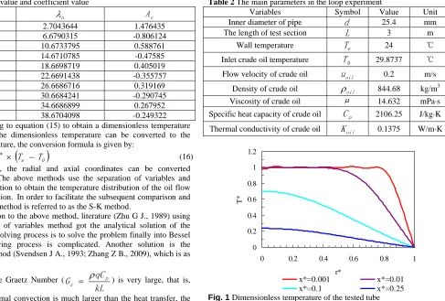
In the wax deposition loop experiment, wax deposition will appear in the test section, so the temperature distribution is mainly calculated around the test section, and the parameters used in the calculation are as shown in Table 2, where the size of the loop test device and the physical properties of crude oil are from the wax deposition loop experiment in literature (Li P., 2014).

The temperature distribution of the loop test section is solved according to the S-K method described in Section 2. For convenience, we analysis the dimensionless temperature at 0.001, 0.01, 0.1, and 0.25

of

x

∗, the results are shown in Fig. 1.

Table 2 The main parameters in the loop experiment

Variables Symbol Value Unit

Inner diameter of pipe

d

25.4 mm

The length of test section

L

3 m

Wall temperature

T

w 24 ℃

Inlet crude oil temperature

T

₀ 29.8737 ℃

Flow velocity of crude oil

u

_oil 0.2 m/s

Density of crude oil

ρ

_oil 844.68 kg/m3

Viscosity of crude oil μ 14.632 mPa·s

Specific heat capacity of crude oil

C

p 2106.25 J/kg·K

Thermal conductivity of crude oil

K

oil 0.1375 W/m·K

0 0.2 0.4 0.6 0.8 1 1.2

0 0.2 0.4 0.6 0.8 1

r*

T*

x*=0.001 x*=0.01

x*=0.1 x*=0.25

Fig. 1 Dimensionless temperature of the tested tube

It can be seen from Fig. 1, the temperature near the tube wall

( is closed to 1) is always below the temperature of the main flow

zone (in the center of the pipe, is 0). With the increase of , the

dimensionless temperature gradually decreases. When the is 0.001

and 0.01 respectively, the temperature near the tube wall suddenly decreases, and the temperature changes very fast. Except the position near the pipe wall, the temperature change of the rest (in the radial

direction of the tube) is slightly; when is 0.1 and 0.25, the

corresponding dimensionless temperature is lower, and near the tube wall, the dimensionless temperature decreases more slowly.

∗

r

∗

r

_x

∗

∗

x

∗

x

It is mentioning that when is 0.001 (at the entrance of the test

section), the value of dimensionless temperature fluctuates, but the range of fluctuation is small, and one of the important reasons for this problem is that the number of characteristic value used in the calculation is less, if we take more characteristic value, we can reduce the effect of this fluctuations (Jin W B., 2015).

∗

x

3.2 The actual temperature distribution of oil flow in the

tested tube

According to the formula which non-dimensional temperature is converted to the actual temperature, the actual temperature distribution of the oil flow at different axial positions in the test section can be calculated. The temperature distributions of the axial distance of 1.1019 meters, 1.7030 meters, 2.3040 meters and 2.9051 meters are given here, as shown in Fig. 2.

of the isothermal interval narrowed, and the temperature of the oil flow began to decrease in the radial direction.

24 25 26 27 28 29 30 31

0 0.002 0.004 0.006 0.008 0.01 0.012 0.014

Radial distance/m

T

em

p

er

at

u

re/

℃

x=1.1019

x=1.7030

x=2.3040

x=2.9051

Fig. 2 Actual temperature of tested tube

4.

COMPARISON OF CALCULATED RESULTS OF

THE TWO METHODS

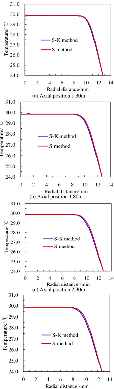
In order to visually find the difference between the S-K method and the Svendsen method, we compare the results of the two methods. The Svendsen method is simply called S method. For convenience, we comparatively analysis the temperature distribution at 1.30 meters, 1.80 meters, 2.30 meters and 2.80 meters from the entrance respectively, the results are shown in Fig. 3.

It can be seen from Fig. 3 that the temperature distribution of the two methods is consistent, that is, the oil flow has an isothermal interval in the radial position and the temperature change near the tube wall is faster. Therefore, the temperature gradient near the wall is larger, which is similar to the actual pipeline.

According to the calculated results, the results obtained by the S method are generally higher than the S-K method. At 1.30 meters and 1.80 meters from the entrance, the difference of the results of two

methods is small, and the maximum difference is 0.23 ℃ and 0.24 ℃

respectively; At 2.30 meters and 2.80 meters from the entrance, the difference of the results of two methods is relatively large, and the

maximum difference is 0.26 ℃ and 0.27 ℃ respectively, that is, the

maximum difference away from the entrance is slightly larger than that the maximum difference near the entrance. On the whole, the difference of temperature distribution in the test section obtained by the two methods is acceptable and well matched.

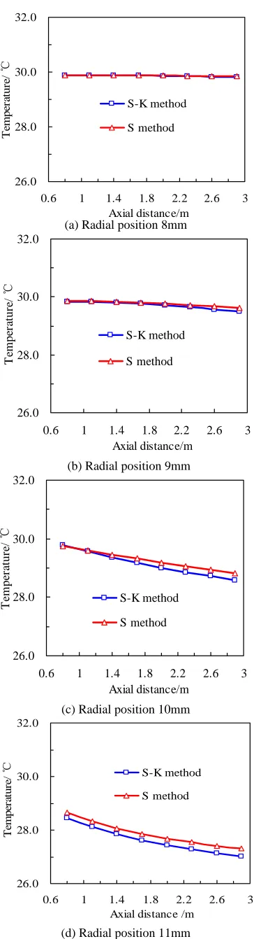
In order to further analyze the difference of the results of two methods, we comparatively analysis the temperature where the radial distance from the center of the tube is 8.0mm, 9.0mm, 10.0mm, 11.0mm and different axial position (0.8m, 1.1m, 1.4m, 1.7m, 2.0m, 2.3m, 2.6m, 2.9m) , the results are shown in Fig. 4.

It can be seen from Fig. 4 that the results obtained by the S method are generally higher than the results obtained by the S-K method. With the change of radial position, the difference is different. The difference of results of two methods is larger at the radial position of 11mm. At the radial position of 8mm and 9mm, the difference of results of two methods is very small, and the maximum difference (2.9 meters) is 0.03

and 0.12 respectively; at the radial position of 10

℃ ℃ mm and 11mm

the difference of results of two methods is relatively larger, and with the increase of the axial distance, this difference becomes relatively

obvious, and the maximum difference is 0.24 ℃ and 0.27 ℃

respectively when the axial distance is 2.9 meters. On the whole, at different radial positions, with the change of axial distance, the results obtained by the two methods are well matched.

24.0 25.0 26.0 27.0 28.0 29.0 30.0 31.0

0 2 4 6 8 10 12 14 Radial distance/mm

T

em

p

er

at

u

re/

℃

S-K method

S method

(a) Axial position 1.30m

24.0 25.0 26.0 27.0 28.0 29.0 30.0 31.0

0 2 4 6 8 10 12 1

Radial distance/mm

T

em

p

er

at

u

re

/

℃

4 S-K method

S method

(b) Axial position 1.80m

24.0 25.0 26.0 27.0 28.0 29.0 30.0 31.0

0 2 4 6 8 10 12 1

Radial distance /mm

T

em

p

er

at

u

re/

℃

4 S-K method

S method

(c) Axial position 2.30m

24.0 25.0 26.0 27.0 28.0 29.0 30.0 31.0

0 2 4 6 8 10 12 1

Radial distance /mm

T

em

p

er

at

u

re/

℃

4 S-K method

S method

(d) Axial position 2.80m

26.0 28.0 30.0 32.0

0.6 1 1.4 1.8 2.2 2.6 3 Axial distance/m

T

em

p

er

at

u

re/

℃

S-K method

S method

(a) Radial position 8mm

26.0 28.0 30.0 32.0

0.6 1 1.4 1.8 2.2 2.6 3

Axial distance/m

T

em

p

er

at

u

re/

℃

S-K method

S method

(b) Radial position 9mm

26.0 28.0 30.0 32.0

0.6 1 1.4 1.8 2.2 2.6 3

Axial distance/m

T

em

p

er

at

u

re/

℃

S-K method

S method

(c) Radial position 10mm

26.0 28.0 30.0 32.0

0.6 1 1.4 1.8 2.2 2.6 3

Axial distance /m

T

emp

er

at

u

re/

℃ _{S-K method}

S method

(d) Radial position 11mm

Fig. 4 Comparison of calculated results of the two methods at different radial positions from the center of the tube

5.

THE DIFFERENCES BETWEEN CALCULATED

RESULTS OF THE TWO METHODS AND

EXPERIMENTAL RESULTS

In order to further verify the rationality of results of two methods, using the two methods, the average temperature at the exit section of the test section is calculated respectively based on the loop test data of Table 2, and the results are compared with outlet temperature (experiment measured) in the test section given in literature (Li P., 2014), the results are shown in Fig. 5.

26 27 28 29 30

S-K method Experimental result

S method

T

em

p

er

at

u

re/

℃

Fig. 5 Comparison of calculated results of the two methods and experimental results

It can be seen from Fig. 5 that the difference between the results obtained by the two methods is smaller, and are slightly higher than the experimental results, and the results obtained by the S method are the largest. In contrast, the results obtained by S-K method are much closer to the experimental results. S-K method avoids solving the numerical integration (S method) and the inconvenience of Bessel function, and it has some superiority.

6.

CONCLUSION

(1) By introducing the dimensionless variable, the energy balance equation is solved by S-K method, and the temperature distribution of the loop test section is obtained (no wax deposition in the wall, constant wall temperature boundary). The results show that there is an isothermal interval in the radial direction of oil flow in the test section at different axial positions, and the oil flow temperature is decreasing near the pipe wall. Therefore, the results obtained by that method are similar to the regularity of actual pipeline; when use S-K method to solve the problem, the calculated value has a small fluctuation in the isothermal internal near the entrance, which does not affect the use of that method, and this fluctuation problem can be avoided by changing the number of characteristic values.

(2) The difference of results between the S-K method and the Svendsen method is compared and analyzed, the results show that the temperature distribution regularity obtained by the two methods is consistent, and the results of the Svendsen method is basically higher than the results of the S-K method. At different axial distances, with the increase of the axial distance, the maximum difference of different radial positions obtained by the two methods increases, and the

maximum difference is 0.27 ℃; At different radial distances , with the

increase of the axial distance, the difference of results obtained by the two methods increases, and the larger the radial distance, the more

obvious the difference, where the maximum difference is 0.27 ℃. From

the difference of the calculated results, the results of the two methods are well matched.

ACKNOWLEDGE

This work was supported by the Special Funding Project of Shaanxi Province Industrial Science and Technology Project (NO. 2015GY094) and Xi'an Petroleum University Youth Science and Technology Innovation Fund (NO. 2015BS011), so grateful here.

NOMENCLATURE

0

T

inlet crude oil temperature, ℃

0

u

average velocity of oil flow, m/s

w

T

the temperature of tube wall, ℃

n

A

the corresponding coefficient, dimensionless

n

λ

Eigenvalues value, dimensionless

0

r

the pipe radius, mm

∗

T

dimensionless temperature variable, dimensionless

∗

r

dimensionless tube radius variable, dimensionless

*

x

dimensionless tube distance variable, dimensionless

e

R

Reynolds Number, dimensionless,

Pr

Prandtl Number, dimensionless,

max

u

the maximum speed of oil flow, m/s

L

the length of test section, m

d

inner diameter of tube, mm

oil

u

oil flow velocity, m/s

p

C

specific heat capacity of crude oil, J/kg·K

oil

K

thermal conductivity of crude oil, W/m·K

z

G

Graetz Number, dimensionless

Greek Symbols

oil

ρ

density of crude oil, kg/m3

β

the relation coefficient, dimensionless,

max

2

u

R

α

β

=

α the relation coefficient which indicating the thermal diffusivity

of the fluid, dimensionless,

p

C

ρ

λ

α

=

λ

the thermal conductivity of the fluid, W/(m·K)

μ the dynamic viscosity coefficient of crude oil, mPa·s

ρ

fluid density, kg/m3

φ

the correction coefficient of droplet growth, generally,

φ

=9

REFERENCES

Azevedo L F A, Teixeira A M., 2003, “A Critical Review of the

Modeling of Wax Deposition Mechanisms,” Petroleum Science and

Technology, 21(3-4): 393-408.

http://dx.doi.org/10.1081/LFT-120018528

Amine, B., Maurel, P., Agassant, F. C., Darbouret, M., Avril, G., Peuriere, E., 2008, “Wax Deposition in Pipelines: Flow-Loop

Experiments and Investigations on a Novel Approach,” SPE Annual

Technical Conference and Exhibition. Society of Petroleum Engineers.

https://doi.org/10.2118/115293-MS

Bern P A, Withers V R, Cairns R J R., 1980, “Wax Deposition in Crude

Oil Pipelines,” European offshore technology conference and exhibition,

Society of Petroleum Engineers.

https://doi.org/10.2118/206-1980-MS

Burger E D, Perkins T K, Striegler J H., 1981, “Studies of Wax

Deposition in the Trans Alaska Pipeline,” Journal of Petroleum

Technology, 33(06): 1075-1086.

https://doi.org/10.2118/8788-PA

Brown T S, Niesen V G, Erickson D D., 1993, “Measurement and

Prediction of the Kinetics of Paraffin Deposition,” SPE annual

technical conference and exhibition. Society of Petroleum Engineers.

https://doi.org/10.2118/26548-MS

Bhat N V, Mehrotra A K., 2005, “Modeling of Deposit Formation from “Waxy” Mixtures via Moving Boundary Formulation: Radial Heat

Transfer under Static and Laminar Flow Conditions,” Industrial &

engineering chemistry research, 44(17): 6948-6962.

https://doi.org/10.1021/ie050149p

Creek, J. L., Lund, H. J., Brill, J. P., Volk, M., 1999, “Wax Deposition

in Single Phase Flow,” Fluid Phase Equilibria, 158(1): 801-811.

https://doi.org/10.1016/S0378-3812(99)00106-5

Edmonds, B., Moorwood, T., Szczepanski, R., Zhang, X., 2007,

“Simulating Wax Deposition in Pipelines for Flow Assurance,” Energy

& Fuels, 22(2): 729-741.

https://doi.org/10.1021/ef700434h

Eskin D, Ratulowski J, Akbarzadeh K., 2014, “Modeling Wax

Deposition in Oil Transport Pipelines,” The Canadian Journal of

Chemical Engineering, 92(6): 973-988.

https://doi.org/10.1002/cjce.21991

ELTON HUNT J R., 1962, “Laboratory Study of Paraffin Deposition,”

Journal of Petroleum Technology, 11: 1259-1269.

http://dx.doi.org/ 10.2118/279-PA

Hsu J J C, Santamaria M M., Brubaker J P., 1994, “Wax Deposition of

Waxy Live Crudes under Turbulent Flow Conditions,” SPE Annual

Technical Conference and Exhibition. Society of Petroleum Engineers.

http://dx.doi.org/10.2118/28480-MS

Huang, Q., Zhang, J., Gao, X., Zhang, Z., 2006, “Study on Wax

Deposition of Daqing Crude Oil,” Acta Petrolei Sinica, 27(4): 125-129.

Handal A D., 2008, “Analysis of Some Wax Deposition Experiments in

a Crude Oil Carrying Pipe,” Ph.D. Thesis, Norway: University of Oslo.

Huang Q Y , Li Y X, Zhang J J., 2008, “Unified Wax Deposition

Model,” Acta Petrolei Sinica, 29(3): 459-462.

http://doi.org/10.7623/syxb200803030

Hoffmann R, Amundsen L., 2009, “Single-Phase Wax Deposition

Experiments,” Energy & Fuels, 24(2): 1069-1080.

https://doi.org/10.1021/ef900920x

Huang, Z., Lee, H. S., Senra, M., Scott Fogler, H., 2011, “A Fundamental Model of Wax Deposition in Subsea Oil Pipelines,”

AIChE Journal, 2011, 57(11): 2955-2964.

http:// doi.org/10.1002/aic.12517

Huang, Z., Senra, M., Kapoor, R., Fogler, H. S., 2011, “Wax

Deposition Modeling of Oil/Water Stratified Channel Flow,” AIChE

Journal, 57(4): 841-851.

http://doi.org/10.1002/aic.12307

Jennings D W, Weispfennig K., 2005, “Effects of Shear and Temperature on Wax Deposition: Coldfinger Investigation with a Gulf

of Mexico Crude Oil,” Energy & fuels, 19(4): 1376-1386.

Jiang B L., 2010, “Research on the Model of Wax Deposition,” Ph.D. Thesis, Qingdao: China University of Petroleum.

Jin W B., 2015, “Study on the Wax Deposition and Prediction Method

of Waxy Crude Oil,” Ph.D. Thesis, Chengdu: Southwest Petroleum

University.

Kok M V, Saracoglu R O., 2000, “Mathematical Modelling of Wax

Deposition in Crude Oil Pipelines (Comparative Study),” Petroleum

science and technology, 18(9-10): 1121-1145.

http://dx.doi.org/10.1080/10916460008949895

Lashkarbolooki M., 2011, “Experimental Study of Oil Deposition

through a Flow Loop,” Journal of Dispersion Science and Technology,

32(3): 312-319.

http://dx.doi.org/10.1080/01932691003659668

Liu Y, Wang Z H, Cheng Q L, Li Y C., 2012, “The Study of Pipeline Wax Deposition Law and Pigging Period for DaQing Waxy Crude Oil,”

Acta Petrolei Sinica, 33(5): 892-897.

http://doi:10.7623/syxb201205023

Li P., 2014, “The Study on Wax Deposition of JingXian Crude Oil

Pipeline,” M.Sc. Thesis, Qingdao: China University of Petroleum.

Li, S., Huang, Q., Wang, W., Wang, C., Ding, Z., 2014, “Experimental Investigation of Wax Deposition at Different Deposit Locations through

a Detachable Flow Loop Apparatus,” 10th International Pipeline

Conference, Calgary, Canada.

https://doi.org/10.1115/IPC2014-33007

Noville I, Naveira L ., 2012, “Comparison between Real Field Data and

the Results of Wax Deposition Simulation,” SPE Latin America and

Caribbean Petroleum Engineering Conference. Society of Petroleum Engineers.

https://doi.org/10.2118/152575-MS

Ramirez-Jaramillo E, Lira-Galeana C, Manero O., 2004, “Modeling

Wax Deposition in Pipelines,” Petroleum science and technology,

22(7-8): 821-861.

http://dx.doi.org/10.1081/LFT-120038726

Svendsen J A., 1993, “Mathematical Modeling of Wax Deposition in

Oil Pipeline Systems,” AIChE Journal, 39(8): 1377-1388.

https://doi.org/10.1002/aic.690390815

Singh P, Fogler H S, Nagarajan N., 1999, “Prediction of the Wax Content of the Incipient Wax-Oil Gel in a Pipeline: An Application of

the Controlled-Stress Rheometer,” Journal of Rheology, 43(6):

1437-1459.

http://dx.doi.org/10.1122/1.551054

Singh, A., Lee, H. S., Singh, P., Sarica, C., 2011, “Flow Assurance: Validation of Wax Deposition Models Using Field Data from a Subsea

Pipeline,” Offshore Technology Conference.

https://doi.org/10.4043/21641-MS

Sadra K B F, Mohsen V S, Shahram M., 2014, “Wax Deposition in Oil

Pipelines Combined with the Wax Precipitation Kinetics,” Petroleum

Research, 24(77): 89-99.

Tian, Z., Jin, W., Wang, L., Jin, Z., 2014, “The study of temperature profile inside wax deposition layer of waxy crude oil in pipeline,”

Frontiers in Heat and Mass Transfer (FHMT), 5(1).

http:// doi: 10.5098/hmt.5.5

Weingarten J S, Euchner J A., 1988, “Methods for Predicting Wax

Precipitation and Deposition,” SPE Production Engineering, 3(01):

121-126.

https://doi.org/10.2118/15654-PA

Wang P Y, Wang W, Gong J, Zhou Y X, Yang W, Zhang Y., 2013, “Effect of Pour Point on Wax Deposition under Static Cooling

Conditions,” Asia-Pacific Journal of Chemical Engineering, 8(5):

749-755.

http:// doi.org/10.1002/apj.1718

Wang W D, Huang Q Y., 2014, “Prediction for Wax Deposition in Oil

Pipelines Validated by Field Pigging,” Journal of the Energy Institute,

87(3): 196-207.

https://doi.org/10.1016/j.joei.2014.03.013

Wang, W., Huang, Q., Liu, Y., Sepehrnoori, K., 2015, “Experimental

Study on Mechanisms of Wax Removal during Pipeline Pigging,” SPE

Annual Technical Conference and Exhibition. Society of Petroleum Engineers. (2015).

https://doi.org/10.2118/174827-MS

Yang F, Zhao Y S, Sjöblom J, Li C X, Paso K G., 2014, “Polymeric Wax Inhibitors and Pour Point Depressants for Waxy Crude Oils: A

Critical Review,” Journal of Dispersion Science & Technology, 36(2):

213-225.

http://dx.doi.org/10.1080/01932691.2014.901917

Zhu G J., 1989, “Engineering Heat and Mass Transfer,” Beijing:

Aviation Industry Press.

Zhang Z B., 2009, “Wax Deposition Property of Waxy Oil in Pipeline,”

Ph.D. Thesis, Qingdao: China University of Petroleum.

Zhou Y X, Gong J, Wang P Y., 2016, “Modeling of Wax Deposition

for Water-in-Oil Dispersed Flow. Asia-Pacific Journal of Chemical

Engineering, 11(1): 108-117.

http://doi.org/10.1002/apj.1948

Zheng, S., Saidoun, M., Palermo, T., Mateen, K., Fogler, H. S., 2017, “Wax Deposition Modeling with Considerations of Non-Newtonian

Characteristics: Application on Field-Scale Pipeline,” Energy & Fuels.

31(5).