Dynamic Models of Learning that Characterize Parent-Child Exchanges Predict Vocabulary Growth

(1)

ISSN 2324-805X E-ISSN 2324-8068 Published by Redfame Publishing URL: http://jets.redfame.com

Dynamic Models of Learning that Characterize Parent-Child Exchanges

Predict Vocabulary Growth

David R Ober1, John A Beekman1

1

Ball State University, United States

Correspondence: David R Ober, Ball State University, United States

Received: November 26, 2015 Accepted: December 30, 2015 Online Published: January 12, 2016

doi:10.11114/jets.v4i4.1215 URL: http://dx.doi.org/10.11114/jets.v4i4.1215

Abstract

Cumulative vocabulary models for infants and toddlers were developed from models of learning that predict trajectories associated with low, average, and high vocabulary growth rates (14 to 46 months). It was hypothesized that models derived from rates of learning mirror the type of exchanges provided to infants and toddlers by parents and caregivers. Slow and rapid growth models assume that rates of acquiring new vocabulary are proportional to (a) the child's current vocabulary and (b) the difference between maximum achievable vocabulary and the child's current vocabulary. These models produce (a) exponential growth and (b) bounded exponential growth, respectively. The third model (interactive engagement) results from the interaction of the two previous models and describes vocabulary growth trajectories with a logistic function. It describes the three empirical growth trajectories for average, slow, and rapid growth in the 14 to 46 month study, and for percentile growth rate trajectories of infants and toddlers between 16 and 30 months in a second study. A substantive outcome to the interactive engagement model is that it provided physically meaningful predictions when it was extended forward in time to 60 months and backward in time to 10 months. Although meaningful predictions of achievement can be made based on polynomial growth models (quadratic, and cubic) that fit empirical data, physically meaningful growth trajectories are obtained for logistic-model predictions beyond the empirical data. Excellent agreement between empirical data and model predictions provide evidence that additional birth through age three exchanges by parents and caregivers will narrow socioeconomic status gaps.

Keywords: child development, dynamic learning models, vocabulary trajectories, socioeconomic status

1. Introduction

It is unreasonable to expect that equal educational outcomes will occur for all students when all students do not arrive at the beginning of their public school education with comparable vocabulary skills. Identifying and treating the root causes of poor academic achievement are much more cost effective than treating students' later educational deficiencies. In order to remedy the wide range of school readiness skills for children prior to their entry into kindergarten, parents and caregivers must be made aware of the vocabulary growth strategies that are needed to prepare children for successful educational experiences, particularly when these practices need to begin at birth.

Early studies have shown that birth through age 5 (B5) cumulative vocabulary growth trajectories are influenced by parental speech and socioeconomic status (SES) effects (Huttenlocher, Haight, Bryk, Seltzer, & Lyons, 1991, Fenson et al., 1994, and Hart & Risley, 1995). A more recent study by Rowe, Raudenbush, and Goldin-Meadow (2012) further demonstrated that 54-month vocabularies were predicable on the basis of 30-month vocabulary learning rates and associated changes in these rates. In this investigation it will be shown that B5 cumulative vocabulary growth trajectories are also characteristic of the types of interaction and communicative techniques used by parents and caregivers. These findings will support the implementation of programs for training parents before the birth of their child with strategies that are known to promote rich vocabularies and to assist parents in the immediate use of these strategies after the birth of the child.

(2)

been used for quite some time to predict vocabulary trajectories for young children (Huttenlocher et al., 1991, and Hart & Risley, 1995).

In the research by Fenson et al. (1994) and Rowe et al. (2012), the different shapes of cumulative vocabulary growth trajectories of infants and toddlers reveal that there are at least three typical shapes that can be associated with low, average, and high vocabulary growth between 16 and 30 months and between 14 and 46 months, respectively. The trajectories associated with average performances are often S-shaped and they can be represented by logistic or cubic functions. The trajectories associated with low and high vocabulary growth rates appear to have quadratic function shapes for which the square terms are positive and negative, respectively. For the studies by Fenson et al. (1994) and Rowe et al. (2012), the vocabulary trajectories were fitted using both logistic and cubic functions and cubic functions, respectively.

In this study we will first show that all three of these characteristic vocabulary trajectory shapes have equations that are derivable from deterministic models of learning as suggested by Rogosa, Brandt, and Zimowski (1982). Specifically the dynamic models of learning proposed by Bao (2007) and Pritchard, Lee, and Bao (2008) will be applied to determine which mathematical functions best fit the typical shapes associated with low, average, and high vocabulary growth. {The models of Bao (2007) and Pritchard et al. (2008) have successfully predicted the learning gains for different types of classroom instruction in university courses.} Secondly, we will use these models to predict three vocabulary growth trajectories reported by Rowe et al. (2012). These three trajectories represent the trajectory of the group mean (n=62), and two additional trajectories that enveloped the range of the maximum and minimum empirical trajectories for the 62 students of their sample. We will then discuss how the three models that predict the Rowe et al. (2012) trajectories are characteristic of the communicative exchanges between children and their parents and caregivers. The final portion of the paper will consist of a discussion of how the results of this study support specific types of intervention strategies for parents and caregivers to utilize during the B5 time span.

1.1 Review of the Literature

Over the past two decades, improvements in technology have made it possible to gather parent-child data quicker and with less effort. Similar advances in computing power and in the handling of large amounts of data have made it possible to analyze the vocabulary trajectories of infants and toddlers and to search for models that not only allow the prediction of trend data but also have models which have theoretical bases associated with teaching and learning. Therefore, the following discussion of the literature will pay particular attention to the models that researchers have used to analyze and predict individual vocabulary growth for infants and toddlers.

Huttenlocher et al. (1991) reported that the amount of early talking by parents to their children and toddlers was significant to their cumulative vocabulary development. In their study of 22 urban-community and middle-class children between the ages of 14 and 26 months, the researchers divided the parent-child pairs into two groups of equal sizes; one group was observed six or seven times at two-month intervals using audio tape recordings and the other group was videotaped three times at four-month intervals. Data from both groups were analyzed with a hierarchical linear model (HLM) to predict growth trajectories for each child. Results of their studies showed that the amount that mothers speak to their children influences the vocabulary growth of the child. The authors clearly stated that their choice of a quadratic function for fitting the data was to measure the acceleration of vocabulary development for the children in their study. At some point after 26 months (the end of their range of data) a deceleration will occur and that will produce an S-shaped vocabulary growth curve over a longer age range for children in their sample.

Fenson et al. (1994) used two MacArthur Communicative Development Inventories (CDIs) to demonstrate that the developmental trajectories of vocabulary production for children between the ages of 8 and 30 months progress at widely varying rates. One of the inventories is for 8-16 month-old infants and the other is for 16-30 month-old toddlers. The work for this study extended over a period of 20 years and used parent reported data from 1803 families. Developmental measures including vocabulary growth were studied by using both empirical data and smoothed-fitted data. Longitudinal growth curves were studied for percentile data at the 10th, 25th, 50th, 75th, and 90th percentiles. Trends associated with vocabulary growth and other measures reveal that the highest, average, and lowest percentile trends have different shapes suggesting the presence of different types of developmental instruction in home environments. Linear, quadratic, cubic, and logistic functions were examined to determine what gave best fits to their data, and the logistic function produced the best fits.

(3)

approximately six years of analysis, the authors determined a wide variation in the average vocabularies at age 36 months of children in upper, middle, and lower SES families as they had average cumulative vocabularies of 1,116, 749, and 525 words, respectively. An even more significant finding was that the children from professional families heard on average about 2,153 words per hour from their parents while children from working class and welfare families heard on average 1,251 and 616 words per hour, respectively, from their parents. The cumulative differences in the amount of language experience acquired by the average children in these three home environments become quite apparent: the average child in the welfare, working-class, and professional families will have heard about 13 million, 26 million, and 45 million spoken words, respectively. The difference between the language experiences of children from professional and welfare families is more than 30 million spoken words heard at 48 months. This gap in words heard prior to kindergarten entry is often referred to as a 30-million word catastrophe [emphasis added].

Rowe, M., Pan, B., and Ayoub, C. (2005) and Pan, B., Rowe, M., Singer, J., and Snow, C. (2005) used the same data set to study maternal input patterns over time and to model individual vocabulary growth for a sample of 108 children in low-income families, respectively. In the study by Rowe et al. (2005) maternal input associated with word types and the amounts of input (talkativeness) were examined to determine whether variability across mothers could be predicted by maternal characteristics. The study by Pan et al. (2005) investigated whether the variables they used to predict rates of change and cumulative vocabulary production were the same as those used for middle-class children. The parent-child sample used in the study was taken from rural New England and all children had been participants in the national longitudinal evaluation of the Early Head Start program. Half of the students were in the EHS program and half were in the control group. The sample was predominately White (91%) and English was the language spoken in 99% of the families. Three sets of videotaped child-parent data were gathered when the children were at about the ages of 14, 24, and 36 months. The number of children-parent pairs observed for three, two, or one observations were 57, 27, and 24, respectively. Since a multilevel growth modeling procedure was used, it was possible to use all of the data even though participants in the study had different numbers of observations and different intervals of time between observations.

After investigating quadratic and logarithmic individual growth model functions the quadratic model was chosen. The average vocabulary production for this sample of 108 low-income children was about 1, 28, and 68 words at 14, 24, and 36 months, respectively. Although the variety in types of words that mothers used with their children was related to predicting vocabulary growth, the numbers of words spoken by the mother alone did not affect vocabulary production. The previously mentioned middle-class studies by Huttenlocher et al. (1991) and multi-SES groups studied by Hart and Risley (1995) did report correlations with the numbers of words spoken by the mother and the child's vocabulary production.

In the study by Rowe et al. (2012) nine cumulative vocabulary measurements were made at four-month intervals for 62 infants and toddlers while they were between the ages of 14 and 46 months. The families in the study were from the Chicago area and they had an average annual income of nearly $60,000 at the start of the project. The ethnicity and races of the families and children studied were 15% Hispanic, 19% Black, 57% White, and 10% other races. The parents had an average education level of 16 years and eight of the families were headed by single-parents mothers. The researchers used SES measures for the family and characteristics of the children in HLM analyses to predict cubic vocabulary trajectories for the children; using these models and growth rates at 30 months, vocabularies of the children were predicted at 54 months.

2. Method

2.1 Data Sources

(4)

Figure 1a. Empirical growth trajectories from Rowe et al. (2012) for the lowest (Min.), average (Mean), and highest (Max.) rates of vocabulary development of infants and toddlers between the ages of approximately 14 and 46 months. The trajectories are centered at 30 months and the solid lines represent the cubic model predictions.

Word production vocabulary trajectory data for children of ages between 16 and 30 months are presented in Figure 1b for the CDI data of Fenson et al. (1994). The data presented are for the children scoring at the 10th, 25th, 50th, 75th, and 90th percentiles and were taken from Fenson et al. (1993). The authors used a logistic model to smoothen their data.

2.2 The Physical Interpretations of Linear, Quadratic, and Cubic Growth Models

When one explores growth curves, linear models are typically chosen first to determine if a simple regression (with a slope and intercept) will describe the data under study and allows one to predict into the future. For these models the slope and intercept are interpreted as its rate of change and an initial value of the variable under study, respectively. For example, in a study of cumulative growth trajectories for infants and toddlers, these quantities will be the number of words in a child's vocabulary at a particular initial time and the number of words added per unit of time.

Education researchers (Rowe et al., 2012) have often referred to this slope (rate of change in vocabulary per unit of time) as a velocity. In those cases where this velocity is not constant and experiences changes, the rate of change in the velocity is referred to as acceleration. Velocity and acceleration are terms from kinematics that are used to describe the motions of objects. When one has knowledge of the forces causing the motion, then one is able to use Newton's second law to determine the position, velocity, and acceleration as functions of time. Therefore, the trajectories of vocabulary (in words) and their rates of change (velocity and acceleration) are analogous to kinematic terms we use daily.

Figure 1b. The CDI word production vocabulary trajectories from Fenson et al. (1993,1994) for girl toddlers and boy toddlers at the 5th, 25th, 50th, 75th, 95th, and 99th percentiles between the ages of 16 and 30 months. The trajectories are centered at 30 months, and both the data points and the solid lines represent logistic model predictions.

Constant acceleration models (associated with constant net forces) are used in mathematics, physics, and engineering to describe both real-world phenomena (for example free fall due to gravity) and approximations to these phenomena. Models with changing accelerations can be incorporated into the models just described. Linearly changing accelerations will have a different physical meaning. In addition there are different characteristic curves associated with the predictions of position in kinematics or of the cumulative vocabulary growth trajectories in child development models.

In Figure 1a are three cumulative growth trajectories from the work of Rowe et al. (2012) for the mean, lowest, and highest cumulative word types of the 62 children (ages 14 - 46 months) where trajectories were labeled M (mean), Min. (minimum), and Max. (maximum). The solid trend lines for the three sets of data are cubic functions; the analyses in

0 200 400 600 800 1000 1200 1400

-20 -15 -10 -5 0 5 10 15 20

C u m u la ti ve W o rd T yp e s

Age - 30 months

Min., Mean, and Max. Growth Trajectories vs. (Age - 30) Months - Cubic Predictions

Max Mean Min 0 100 200 300 400 500 600 700

-20 -15 -10 -5 0 5 10 15 20

N u m b e r o f W o rd s P ro d u ce d (M ax im u m = 6 8 0 )

(Age - 30) months

CDI - Production Vocabulary vs. Age (months) by Percentile for Girls - Logistic Smoothed (16 - 30)

99th 95th 75th 50th 25th 5th 0 100 200 300 400 500 600 700

-20 -15 -10 -5 0 5 10 15 20

(Age -30) months

CDI - Production Vocabulary vs. Age (months) by Percentile for Boys - Logistic Smoothed (16-30)

(5)

their study used a cubic model and its associated 30-month velocities and accelerations to make vocabulary predictions at 54 months. Presented in Appendix A1 Figures A1a and A1b are the velocities and accelerations, respectively, for the three data sets, the mean, minimum, and maximum over the 14- through 46-month time period assuming cubic cumulative vocabulary functions.

2.3 Dynamic Vocabulary Growth Models Based on Theories of Learning

The logistic growth function (gamma process) model of Bao (2007) and Pritchard et al. (2008) will be shown to be the inclusive model of choice in this study; the authors also refer to it as the interactive engagement model. This model incorporates two growth functions, the exponential growth function (beta process) and limited exponential growth function (pure memory alpha process), that predict slow and rapid growth, respectively. The logistic model predicts average growth as well as the slow and rapid growth extremes. Before introducing the differential equations associated with these three growth models, we call attention to the mathematical derivations and terminology associated with the logistic and exponential growth models presented in Appendix B. These derivations use the logistic and exponential growth function derivations by Keyfitz & Beekman (1984).

2.3.1 The Linear Vocabulary Growth Model and Parents as Tutors

One-on-one tutoring has been used for centuries as both a primary and supplemental method of instruction. When Pritchard et al. (2008) compare the tutor model with their alpha, beta, and gamma process models, they find tutoring to be the most effective learning model. Therefore, infants and toddlers have opportunities to experience this type of instruction in their development of cumulative vocabularies depending on the “teaching methods” used by their parents and caregivers during their B5 development period.

In the tutor model, the parent or caregiver is aware of what the child knows and in the case of vocabulary development the child can learn a fixed amount of vocabulary at regular intervals. If λk is the rate (words per unit time) at which the

k-th child’s cumulative vocabulary Vk increases, following is the differential equation that describes this process:

dVk/dt = λk = constant (1)

The solution to this equation for the cumulative vocabulary Vk (t) as a function of time t is as follows:

Vk (t) = λk (t - t0) (2)

where t0 is the time axis intercept. The velocity dVk/dt for this case is λk (a constant) and the acceleration d2Vk/dt2 is

then zero. Presented in Figure 2 are the predictions of the linear growth (tutor) model for the mean (Mean), minimum (Min.), and maximum (Max.) trajectory data of Rowe et al. (2012).

Figure 2. The tutor model assumes constant rates (velocities) of acquiring vocabulary. This model was applied to the Min., Mean, and Max, cumulative growth trajectories of Rowe et al. (2012) for the 14- to 46 month time periods. For the Min. trajectory, it was analyzed as two consecutive linear growth trajectories that were four and five waves in length.

2.3.2 The Beta Process, an Exponential Growth Model

Bao (2007) designated the beta learning process as the development of new knowledge when the rate of acquiring new knowledge is proportional to the knowledge possessed by the learner. When this process is applied to cumulative vocabulary growth, the rate at which the k-th child’s cumulative vocabulary Vk increases is given by the following

differential equation:

dVk/dt = βk Vk (3)

where βk is a constant that represents the probability per unit time that there is an increase in the student's cumulative

vocabulary. The solution to this differential equation for the cumulative vocabulary Vk(t) as a function of time t is as

follows:

y = 25.7*(x - 15.8) R² = 0.99 y = 24.0*(x - 31.7)

R² = 1.00 y = 1.0*(x - 15.8)

R² = 0.81

0 200 400 600 800 1000 1200 1400

0 10 20 30 40 50

Cu

m

ul

at

ive

W

or

d

Typ

es

Age in Months

Tutor Model - Linear Growth Rates of Min., Mean, and Max. Cumulative Word-Type Trajectories

(13.7 - 47.4 Months)

Max. Mean Min. (4) Min. (5) y = 37.7*(x - 13.7)

(6)

Vk (t) = Vk0 [exp (βk (t - t1)] (4)

where Vk0 is the initial number of words in the student's vocabulary at a time t1 when an initial vocabulary is determined.

Presented in Figure 3 is an exponential growth model prediction applied to the minimum trajectory data (Min.) of Rowe et al. (2012).

In a study of cognitive growth models Van Geert (1991) applied the exponential growth model and several other growth models to vocabulary growth as examples of dynamic cognitive growth models. Huttenlocher et al. (1991) considered using the exponential growth model to fit vocabulary growth data for middle-class children; however, they chose a quadratic model since it provided a better fit to all of their data.

At first glance one would think that exponential growth is a good thing in a vocabulary growth model. However, the beta process in vocabulary development has a small probability for growth when the cumulative vocabulary Vk is small.

For example, a child that is not stimulated verbally by the parent and caregiver will learn predominately by the beta process and develop at a much slower rate with a delayed development. In addition to the early work by Huttenlocher et al. (1991) and Hart and Risley (1995), the small number of parent word types used by parents associated with the minimum vocabulary development was also replicated in the study by Rowe et al. (2012).

2.3.3 The Alpha Process, a Pure Memory Model That Yields Limited Exponential Growth

Bao (2007) designated the alpha instruction process as the direct addition of new knowledge to the learner and the rate of acquiring the new knowledge is proportional to the total possible knowledge to be gained by the learner; Pritchard et al. (2008) referred to the process as the pure memory model. The learning is independent of the learner’s knowledge status. When this process is applied to cumulative vocabulary growth the rate at which the k-th child’s cumulative vocabulary Vk increases is given by the following differential equation:

dVk/dt = αk (Cmax - Vk) (5)

where αk is a constant that represents the probability per unit time that there is an increase in the student's cumulative

vocabulary and Cmax is the maximum attainable vocabulary of the child in this parent's environment; (Cmax - Vk) is

providing the child with words they do not know. The solution to this equation is as follows:

Vk (t) = Cmax - (Cmax - Vk0) [exp (-αk (t - t0))] (6)

where Vk0 is the initial number of words in the student's vocabulary at a time t0 when an initial vocabulary is determined.

Presented in Figure 3 is the growth model that exponentially decreases the difference between the maximum attainable vocabulary Cmax and initial vocabulary Vk0 for the maximum (Max.) trajectory data of Rowe et al. (2012).

In contrast to the exponential growth model (beta process) which best describes slow learners and which likely involves larger amounts of self-learning, the limited exponential growth model (alpha process) is a highly efficient model similar to the tutor model, a model that describes rapid learners and leads to larger vocabularies. We have noted in the work of Hart and Risley (1995) the disparity in the number of words received from parents and caregivers by high and low SES children as the "30-million word catastrophe." A similar SES disparity is present in the data of Rowe et al. (2012) where the word types recorded for parents and caregivers during the 90-minute first-visit observations were 60 and 708 words, respectively, for the minimum (Min.) and maximum (Max.) cumulative vocabularies.

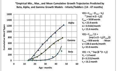
Figure 3. The exponential growth model (beta process), the limited exponential growth model (alpha process), and the interactive engagement model (gamma process) which encompasses the alpha and beta processes to provide logistic growth are shown in the above figure; these models have been used to predict the Min., Max. and Mean cumulative growth trajectories of Rowe et al. (2012), respectively. The respective family variables associated with the slowest (Min.), fastest (Max.), and average (mean) developing trajectories were as follows: 10.0, 18.0, and 15.6 years parent education, $7,500, $100,000, and $59,476 parent income, and 60, 708,and 377 parent word types used during visit 1.

0 200 400 600 800 1000 1200 1400 1600

0 10 20 30 40 50 60

Cu

m

u

la

ti

ve

W

o

rd

T

yp

e

s

Age - months

*Empirical Min., Max., and Mean Cumulative Growth Trajectories Predicted by Beta, Alpha, and Gamma Growth Models - Infants/Toddlers (14 - 47 months)

V(t) = Cmax- (Cmax- V0) * [exp (-α (t - t0))] Cmax= 3038 words V0= 22.8 words α = 0.0160/month t0 = 15.6 months

V(t) = Cmax/ (1 + [exp (-γ (t - t0)/Cmax)]) Cmax= 858 words - Mean γ = 138.6 words/month t0= 32.8 months V(t) = V1* Exp [β *(t - t1)] V1= 1.0 word β = 0.213/month t1 = 16.2 month Beta

(7)

2.3.4 The Gamma Process, an Interactive Engagement Model That Produces Logistic Growth

Bao (2007) and Pritchard et al. (2008) combined the alpha and beta learning processes to formulate a growth model which takes the form of a logistic function. The interaction of these two processes in a classroom environment promotes interactive engagement (Hake, 1998). In this model, the direct addition of new knowledge to the learner is proportional to the total possible knowledge yet to be gained by the learner and the learner’s current knowledge status. When this process is applied to cumulative vocabulary growth the rate at which the k-th child’s cumulative vocabulary Vk

increases is given by the following differential equation:

dVk/dt = γk Vk (Cmax - Vk) (7)

where γk is a constant that represents the probability per unit time-word that there is an increase in the student's

cumulative vocabulary and Cmax is the maximum attainable vocabulary of the child in this parent’s home environment.

The solution to this equation is as follows:

Vk (t) = Cmax /(1 + {exp (-γk (t - t0)/Cmax)}) (8)

where t0 is the time at which Vk (t) has a value of Cmax/2 and it is the inflection point of the trajectory. Presented in

Figure 3 is the characteristic S-shaped logistic curve that exponentially increases until reaching a point of inflection where it then continues to approach a maximum attainable vocabulary Cmax for the mean (M) trajectory data of Rowe et

al. (2012).

We also point out that the solution to Equation 7 can also be expressed in a different form by evaluating the constants of integration in a different manner. If one chooses Vk0 as the initial number of words in the student's vocabulary at a

time t0 when an initial vocabulary is determined, the solution to Equation 7 is as follows:

Vk (t) = Cmax /(1 +[(Cmax - V0)/V0)] ∙{exp (-γk Cmax (t - t0))}). (8a)

The values obtained for Cmax are the same for Equations 8 and 8a, however, the time t0 associated with Equation 8

represents the inflection point at one half of Cmax which is when the maximum velocity and zero acceleration occur.

This measure of time t0 gives one an opportunity to quickly compare the time lags in cumulative vocabulary

development between the rapid learners and the toddlers that develop at delayed and slower rates.

3. Results

In their paper on growth curve analysis Rogosa et al. (1982) noted that depending upon the discipline, measures of change were typically expressed as polynomial functions or as solutions to differential equations of the rate of change of the measure. In either case, most research studies are conducted using one single model to analyze all data in the study. The use of terms like velocity and acceleration by Rowe et al. (2012) prompted us to consider both types of models. We investigated models that predict future vocabularies of infants and toddlers, and we considered models that attach instructional strategies used by parents and caregivers to the shapes of the growth curves.

The data presented in the study by Rowe et al. (2012) contain a diverse SES sample and the nine observations made for each of the 62 participants in their 32-month study span an age range (14-46 months) that provide well defined mean, high, and low trajectories. The association of these three trajectories with levels of achievement and parent or caregiver exchanges makes these three data sets excellent candidates for study using both polynomials and different types of instruction models.

As we present the results of our analyses, we will address the physical interpretations of both the polynomial and dynamic models for the three data sets (Mean, Min., and Max) of the Rowe et al. study. We will present results for the linear and cubic models of cumulative word-type trajectories. These examples will be considered with their analogous kinematic descriptions for the motion of particles in dynamic systems typically governed by Newton’s laws.

3.1 Velocity and Acceleration in the Tutor and Cubic Growth Models

Presented in Figure 2 and in Table 1 are the results of analyses for the tutor model’s linear fits to the Mean, Min., and Max. data sets of Rowe et al. (2012). Equation 2 provides a rate of increase (slope/velocity) for vocabulary trajectories and an x intercept associated with an approximate onset of vocabulary development growth. Table 1 summarizes the Max., Mean, and Min. rates of increase as 37.7, 25.7, and 24.0 words/month, respectively; similarly the x intercepts (t0) are 13.7, 15.8, and 31.7, months, respectively.

(8)

30-month cubic equations (see Table 2) are compared to the tutor analyses (Table 1), the Max. velocity results are 36.7 and 37.7 words/month, respectively, while the Min. velocity values are quite different (7.9 and 24.0 words/month, respectively) due to the delay in the onset of cumulative vocabulary production associated with the Min. data set.

The rates of vocabulary increase (velocities) and their associated rates of change (accelerations) for the three vocabulary data sets fitted with cubic functions and just described are presented in Appendix A1 Figures A1a and A1b, respectively. These results were obtained by successive differentiation of the cubic equations presented in Figure 1a and Table 2. The Max. velocity trajectory in Appendix A1 Figure A1a indicates that it decreases from 52.9 words/min at 16.1 month to 36.7 and 33.7 words/month at 30 and 45 months, respectively. During similar time periods the Mean velocity trajectory increases from 7.4 words/month to 29.8 before decreasing to 20.5 words/month for 14.2, 30, and 45 months, respectively, while Min. grows continuously from 0.4 to 7.9 and then 35.0 words/month for 21.5, 30, and 45 months, respectively. While one may think that the Min. velocity trajectory has overtaken the Max. velocity and a student with such a trajectory has finally “caught up,” the cumulative vocabularies are represented by the areas under their respective curves and at 45 months the Max., Mean, and Min. cumulative vocabularies were approximately 1237, 790, and 328 words, respectively.

Table 1. Comparisons of linearly increasing tutor model predictions of cumulative vocabulary (constant velocity) applied to empirical data of Rowe et al. (2012) for highest (Max.), average (Mean), and lowest rates of vocabulary development. Graphical results are presented in Figure 2

Tutor Model Cumulative Vocabulary Development Rates of Change

Variable (Units) Max. Mean Min. Min.

Visits 1-9 Visits 1-9 Visits 1-5 Visits 6-9

Velocity (Words/Month) 37.7 25.7 1.0 24.0

t0 (Months) 13.7 15.8 15.8 31.7

R2 0.993 0.992 0.806 1.000

Table 2. Comparisons of cubic model predictions for cumulative vocabulary applied to empirical data of Rowe et al. (2012) for average (Mean), lowest (Min.) and highest (Max.) rates of vocabulary development. Graphical results are presented in Figure 1a

Cubic Model Variables for Cumulative Vocabulary Development Intercepts, Velocities, Accelerations, and Rates of Change in Accelerations

Variable (Units).Centered at 30 Months

a

Mean Fixed

Effects Model 1 Mean Min. Max.

Intercept (Words) 342.5 345.7 27.4 648.8

Velocity (Words/Month) 30.2 29.8 7.86 36.7

Acceleration

(Words/Month/Month) 0.197 0.188 0.606 -0.352

Acceleration Rate of Change

(Words/Month/Month/Month) -0.025 -0.022 0.013 0.011

R2 0.994 0.999 0.992 0.998

a

Intercept, linear change, quadratic change, and cubic change variables are from Rowe et al. (2012).

Presented in Appendix A1 Figure A1b are the acceleration trajectories associated with the cubic vocabulary trajectories for the Max., Mean, and Min. data sets. The 1.0 word/month/month deceleration of the Max. data set’s initial (large) 53 words/month vocabulary acquisition rate (velocity) in Appendix A1 Figure A1a suggests that prior to the first wave of data that were gathered, a vocabulary spurt took place in which the acceleration was first positive before becoming negative. The Mean data set’s acceleration ranges from about 2.5 words/month/month at approximately 14 months to a deceleration of -1.8 words/month/month at approximately 46 months; the acceleration of zero at approximately 33 months suggests an inflection point for the Mean vocabulary trajectory at that point. The acceleration associated with the Min. data set begins at about 14 months and the acceleration increases to approximately 2.5 words/month/month at 45 months; experience would suggest that the velocity will begin to rapidly decelerate and produce an inflection point in its vocabulary trajectory within the next several months. Knowledge of the velocity and acceleration trajectories provides insight as to when vocabulary spurts occur and their duration.

3.2 Dynamic Models Predict the Slowest, Most Rapid, and Average Growth Rates

In order to address the third item in our Problem Statement we will use the alpha, beta, and logistic models by Bao (2007) and Pritchard et al. (2008) to predict three vocabulary growth trajectories reported by Rowe et al. (2012). The three trajectories are associated with their Max., Mean, and Min. data sets previously discussed.

3.2.1 Initial Exponential Growth Model Is Slowest Growth

(9)

acquisition rates and their trajectories have the latest onsets. The basis for this model assumes that the vocabulary acquisition rate is proportional to current vocabulary of the child. If learners having these trajectories are not stimulated by someone in their environment, self-learning vocabulary growth will occur slowly. As noted earlier exponential growth (the beta process) will not continue to be the dominant process for vocabulary development indefinitely; an interactive engagement (gamma process) will begin to dominate. However, for these children vocabulary development will be delayed in time, their learning rate (velocity) will be slower, and the maximum attainable vocabularies by the children in this environment will be both smaller and limited when compared to the average and children with larger vocabularies due to the smaller vocabularies used by their parents and caregivers (Rowe et al. (2012)).

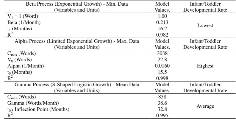
Table 3. The empirical data of Rowe et al. (2012) for the lowest (Min.), the highest (Max.), and the average (Mean) rates of vocabulary development have been fitted by the following three dynamic growth models, respectively: exponential (beta process), exponential decrease of the difference between the current vocabulary and the maximum achievable (alpha process), and the interactive engagement (gamma process)/logistic models

Beta Process (Exponential Growth) - Min. Data (Variables and Units)

Model Values.

Infant/Toddler Developmental Rate

V1 = 1 (Word) 1.00

Lowest

Beta (1/Month) 0.213

t1 (Months) 16.2

R2 0.982

Alpha Process (Limited Exponential Growth) - Max. Data (Variables and Units)

Model Values.

Cmax (Words) 3038

Highest

V0 (Words) 22.8

Alpha (1/Month) 0.0160

t0 (Months) 15.5

R2 0.998

Gamma Process (S-Shaped Logistic Growth) - Mean Data (Variables and Units)

Model Values.

Cmax (Words) 858

Average

Gamma (Words/Month) 38.6

t0.5 Inflection Point (Months) 32.8

R2 0.995

3.2.2 Limited Exponential Growth Provides Most Rapid Growth

Presented in Table 3 and Figure 3 are the results of fitting the Max. empirical data to a limited-growth exponential growth model that is described by Equation 6. The child’s vocabulary acquisition rate is proportional to the difference between a maximum achievable vocabulary provided by the parents and caregivers and the child’s current vocabulary; this difference (see Equation 5) will provide an exponentially decreasing difference (see Equation 6). The Max.’s empirical data set is representative of infants and toddlers with the highest vocabulary acquisition rates and their trajectories have the earliest onsets. Learners having these trajectories are stimulated by parents and caregivers in their environment and this produces a limited maximum growth in a format to the tutor model which is not limited. It is reasonable to assume that this rapid rate of vocabulary acquisition will be slowed as the toddler progresses into a more interactive engagement environment where the self-learning occurs in a more connected manner than pure alpha process (memory method).

3.2.3 Logistic Growth Model Describes Average Vocabulary Growth as Well As Most Rapid and Slowest Growth

Presented in Table 3 and Figure 3 are the results of fitting the Mean empirical data set to a logistic curve which is the solution for an interactive engagement growth model that is described by Equation 8; in terms of the alpha and beta processes previously described, the logistic curve is the solution to a differential equation of the gamma process for learning that is the interaction between the alpha and beta processes.

(10)

Figure 4. The Min., Mean, and Max, cumulative vocabulary trajectories of Rowe et al. (2012) were fitted with the interactive engagement (logistic) model over the time periods of their nine waves of data (14. to 47.4 months). The trajectories were then extended backward in time and forward in time to approximately 58 months.

3.3 Summaries of the Tutor, Alpha, Beta, and Logistic Growth Models

The physical interpretations of the three dynamical models of Bao (2007) and Pritchard et al. (2008) when applied to cumulative vocabulary development are summarized as follows: first, the beta process is the exponential growth model (Equation 4) which provides the slowest vocabulary development rate and it is associated with self-learning rather than stimulation from parents and caregivers; second, the alpha process is the most rapid vocabulary development rate (referred to as the memory model) and it exhibits bounded exponential growth (Equation 6) which results from being exposed by parents and caregivers to the vocabulary that the child does not know; and thirdly, the gamma process is an interactive engagement (IE) model that combines the previous two models into an equation that yields the S-shaped logistic growth model (Equation 8).

The IE model is responsible for most situations where the learner is using input from all sources in the child’s environment as well as the child’s current vocabulary. It should be noted that since Equation 7 contains the alpha and beta process terms, one would expect the logistic model to provide satisfactory if not excellent fits to not only the Mean (average) trajectory, but also to the Min. and Max. trajectories which are described by the beta and alpha processes, respectively (see Table 4 and Figure 4). Presented in Appendix A2 Figure A2a are the velocities predicted by the logistic growth model (Equation 8) for the vocabulary trajectories in Table 4 and Figure 4 for the Min., Mean, and Max. data sets of Rowe et al. (2012).

In Appendix A2 Figure A2a the expected bell-shaped velocity curves which are derived from the three logistic curves for the vocabulary trajectories in Figure 4 demonstrate the differences in the vocabulary developmental rates of the Min., Mean, and Max. trajectories beginning at 10 months. Similarly, the peak developmental rates of these three trajectories are 27.8, 34.6, and 46.8 words/month, respectively, and they occur at 41, 33, and 31 months, respectively, which are also the inflection points in the vocabulary trajectories in Figure 4. One is also reminded that the areas under the curves in Appendix A2 Figure A2a represent the cumulative vocabularies for each trajectory. Not only does this show the largest differences in developmental rates of acquiring vocabularies between the Max. (46.8 words/month) and Min. (27.8 words/month) children, but, their peak rates are also ten months apart by age 40 months. A comparison of the long-term vocabulary average acquisition rates of the linear (tutor) model (Figure 2) and the interactive engagement peak rates (Appendix A2 Figure A2a) for the Min., Mean, and Max. data sets indicate that they scale similarly with one another (24.0, 25.7, and 37.7 words/ month and 27.8, 34.6, and 46.8 words/month, respectively).

0 200 400 600 800 1000 1200 1400 1600

0 10 20 30 40 50 60

Cu

m

u

la

ti

ve

W

o

rd

T

yp

e

s

Age - months

*Gamma Process - Interactive Engagement Model for Max., Mean, and Min. Cumulative Growth Trajectory Predictions - Infants/Toddlers (14 - 47 Months)

V(t) = Cmax/ (1 +

[exp (-γ (t - t0)/Cmax)])

Cmax= 1295 words - Maximum

γ = 187.7 words/month t0= 30.5 months

Cmax= 858 words - Mean

γ = 138.6 words/month t0= 32.8 months

Cmax= 397 words - Minimum

(11)

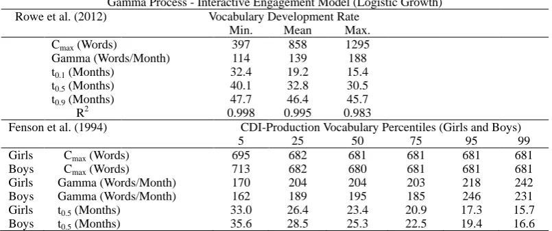
Table 4. Logistic growth model predictions (gamma process) for cumulative vocabulary growth applied to empirical data of Rowe et al. (2012) for lowest (Min.), average (Mean), and highest (Max.) rates of vocabulary development. Similarly the logistic model predictions have been applied to the CDI-production vocabulary percentile trajectories of Fenson et al. (1994); this production vocabulary was measured by a 680-word checklist. t0.1, t0.5 , and t0.9 refer to the times when

vocabularies reach the indicated fractions of Cmax. Graphical results are presented in Figure 4 for the Rowe et al. (2012)

data and Figure 6 for the Fenson et al. (1994) data for girls and boys

Gamma Process - Interactive Engagement Model (Logistic Growth) Rowe et al. (2012) Vocabulary Development Rate

Min. Mean Max.

Cmax (Words) 397 858 1295

Gamma (Words/Month) 114 139 188

t0.1 (Months) 32.4 19.2 15.4

t0.5 (Months) 40.1 32.8 30.5

t0.9 (Months) 47.7 46.4 45.7

R2 0.998 0.995 0.983

Fenson et al. (1994) CDI-Production Vocabulary Percentiles (Girls and Boys)

5 25 50 75 95 99

Girls Cmax (Words) 695 682 681 681 681 681

Boys Cmax (Words) 713 682 680 681 681 681

Girls Gamma (Words/Month) 170 204 204 203 218 242

Boys Gamma (Words/Month) 162 189 195 185 246 231

Girls t0.5 (Months) 33.0 26.4 23.4 20.9 17.3 15.7

Boys t0.5 (Months) 35.6 28.5 25.3 22.5 19.4 16.6

A further test of the logistic-interactive engagement model (gamma process) is to compare the empirical velocities from the empirical data in Figure 4 with the predicted velocities shown in Appendix A2 Figure A2a. These results for the Min., Mean, and Max. data sets are shown in Appendix A2 Figure A2b. The empirical and predicted velocity data trends are in excellent agreement for the Min. and Mean data, but the empirical data trend is unclear without error estimates for the Max. data set.

Figure A3a (Appendix A3) provides the three predicted acceleration curves which are derived from the three velocity trajectories in Appendix A2 Figure A2a. The accelerations rapidly increase, reach maxima, and then decrease to zero followed by decelerations that follow similar changes that approach zero at the same ages. Maximum accelerations for the Max., Mean, and Min. data sets are at 22, 24, and 36 months, respectively, and their respective vocabularies are 286, 167, and 95 words. The accelerations pass through zero at the maximum velocities. Figure A3a (Appendix A3) suggests that vocabulary spurts may have begun prior to the data collection process for the Max. and Mean data sets.

In the same manner that empirical velocities were computed from the data in Figure 4 and then compared with the predicted velocities shown in Appendix A2 Figure A2a, empirical accelerations were computed for the Min., Mean, and Max. empirical data sets of Appendix A2 Figure A2b. Shown in Appendix A3 Figure A3b are the empirical and predicted logistic-interactive engagement model comparisons. The Min. and Mean comparisons are quite encouraging, but the Max. data comparison for acceleration trends is less favorable.

3.3.1 Logistic (Gamma Process) and Pure Memory (Alpha Process) Growth Trajectories Predicted in Simulation Studies

An excellent model for simulating the rate at which a child learns the meaning of a word is contained in McMurray (2007) and Mitchell and McMurray (2008). In that model, a Gaussian distribution is used to model a distribution of word difficulty. This distribution can occur from the influence of many independent distributions and the Central Limit Theorem. Once this distribution is determined, the cumulative growth trajectory V(t) is obtained by integrating the distribution from zero to a specified time t.

Distributions of differing difficulty can be constructed by assigning each word in the distribution the following attributes: Di the degree of difficulty of each word; ri the number of times a word must be heard before being learned (or

its history); and pi the probability that the word is heard by the child during a given time interval. In their original

deterministic model, the researchers used simulations on a 10,000 word lexicon for all pi = 1 and each ri corresponded to

the difficulty Di. Presented in Figure 1B of McMurray (2007) and Figure 2B of Mitchell and McMurray (2008) are the

(12)

In constructing their stochastic model simulations, Mitchell and McMurray (2008) considered two types of simulations by setting the ri equal to 1 (no history) and ri greater than 1 (the previous history associated with learning the word is

important). On the basis of the models presented in this investigation, their stochastic model simulations are consistent with the alpha process (Equation 6) for the r = 1 case and with the interactive engagement logistic growth model (gamma process of Equation 8) for the r > 1 case; the stochastic trajectory predictions for r = 1 and r > 1 are shown in Figures 3 and 4, respectively, of Mitchell and McMurray (2008). As the authors pointed out, their "no history" stochastic predictions show no spurts and in fact have decreasing velocities the same as shown in the alpha process of this study (see Figure 3). Bao (2007) and Pritchard et al. (2008), as pointed out earlier, referred to the alpha process as the "pure memory model" (Equation 6) while the r > 1, past history case, is consistent with the vocabulary (V) term in Equation 8 which multiplies the (Cmax - V) term. The stochastic model of Figure 3 in the Mitchell and McMurray (2008)

paper is approximately fitted by the alpha process (Equation 6) with the following parameters: Cmax = 9160 words, Vk0

= 0 words, t0 = 0 Time Step Units, and α = 0.00033 Words/Time Step.

4. Discussion

4.1 Growth Models Supported by Assumptions from Theories of Learning

Equations 3, 5, and 7 are differential equations for rates of learning that have solutions which predict slow, rapid, and intermediate (average) cumulative vocabulary growth trajectories, respectively. The three sets of empirical data (Min., Max., and Mean) from Rowe et al. (2012) - provided stringent tests of the three dynamic models associated with Equations 3, 5, and 7.

For Equation 3, the beta process, the rate for increasing a child's cumulative vocabulary is proportional to the child's vocabulary at that time and this leads to exponential growth. At first glance one may think this will lead to rapid growth; however, this models a child who creates new words in isolation. Therefore, the solution to this equation leads to slow growth under the conditions described in this study. It should also be noted that once exponential growth does begin, one cannot expect the child to produce new vocabulary indefinitely in an unbounded manner.

Equation 5, the alpha process, has also been identified as the pure memory model. In this model the rate of learning is proportional to the difference between the child's current vocabulary and a maximum vocabulary Cmax that is achievable

in an environment provided by the parents and caregivers that is rich in vocabularies that introduce words that are not known by the child.

Equation 7, the gamma process, is the interaction of the alpha and beta processes; in classrooms, this method of learning is referred to as interactive engagement. Students use their present knowledge in acquiring new knowledge. As in the alpha process, there is a maximum achievable vocabulary Cmax for each student that is dependent upon the environment

provided by the parents and caregiver. One does not expect children to create vocabulary words that they have not heard; the vocabularies of the parents and caregivers and their methods of reinforcement and exchanges in this model are vital in new vocabulary development. This method of learning produces average learning rates. It is likely that all children learn by this model of learning since both the alpha and beta processes are extreme initial applications of the model.

The Min., Mean, and Max. empirical growth trajectory data of Rowe et al. (2012) were analyzed using the beta, gamma, and alpha dynamic models, respectively; the results are presented in Figure 3 and Table 3. The quality of the corresponding cubic-model and dynamic-model fits for each of the three trajectories are quite similar. (It should be noted that the beta process has only three parameters while the other five fits have four parameters.)

The most significant result associated with the dynamic models is the application of the gamma model (logistic growth) to all three sets of empirical data - Min., Mean, and Max. - and obtaining slightly higher quality fits for the Min. and Max. data sets than for the Mean data set (see Figure 4). As noted earlier, the gamma process approximates the beta and alpha processes before and after the inflection points, respectively. It should also be noted that the Cmax variables of the

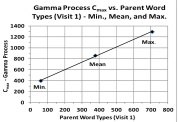
gamma process correlate with the family variables for the Min., Mean, and Max. empirical data sets; particularly significant is the correlation between Cmax and the parent word types (see Figure 5). Cmax for each of the Min., Mean,

(13)

Figure 5. Shown in this figure is the correlation between Cmax values we determined for the Min., Mean, and Max.

growth trajectories (see Figure 4) and the parent word types of visit 1 in the study by Rowe et al. (2012). Cmax is the

maximum achievable word types achievable for the child in the interactive engagement model (gamma process).

4.2 Interactive Engagement Model Predictions of Pace and Acceleration

Equation 8, the interactive engagement (gamma process) model, provides excellent predictions for the Min., Mean, and Max. empirical data (see Figure 4). By taking successive derivatives of the functions in Figure 4, the pace (rate of acquiring vocabulary per unit time) and acceleration for the Min., Mean, and Max data sets are computed, and they are presented in Appendix A2 Figure A2a and Appendix A3 Figure A3a, respectively. The paces reach maxima at the inflection points of the vocabulary trajectories with values of 27.8, 34.5, and 46.8 words/month at 40, 33, and 31 months for Min., Mean, and Max., respectively. (In Figures A2a (Appendix A2) and A3a (Appendix A3) the final empirical data points end between 45 and 47 months although the theoretical curves extend to approximately 60 months.) It is quite plausible that children do experience declining pace prior to school entry unless parents were to make specific efforts to increase the vocabulary development of their children with formal reading and language instruction during this time period.

Rowe et al. (2012) chose not to investigate any vocabulary spurts in their study; they were most interested in predicting the vocabulary skills of their students when they entered kindergarten and this was done on the basis of trajectory information at approximately 30 months. However, it is seen from the interactive engagement model that Appendix A3 Figure A3a predicts maximum accelerations at 22, 24, and 36 months for the Max., Mean, and Min. data sets, respectively. While there is considerable uncertainty as to what part of the acceleration trajectory constitutes a spurt, it is clear that the students with smaller vocabularies lag the average and rapidly developing students by approximately 12 months or more until they reach maximum accelerations.

The 16-30 month CDI production vocabulary trajectories by Fenson et al. (1993, 1994) (see Figure 1b) are the results of data that have been smoothed by fitting it to a logistic function. The authors explicitly stated that they did not understand why the logistic function provided the best fits to their empirical data, but stated that further study of this result was warranted. Therefore, the trajectories for the 5th, 25th, 50th, 75th, 95th, and 99th percentile data for girls and boys (16-30 months) were fitted using Equation 8 (the logistic-interactive engagement model) and in each case unique fits were obtained; these results are included in Table 4. To further test this model, the trajectories were extended back in time to 10 months and forward to 48 months; these results are shown in Figure 6.

Figure 6. The logistic parameters of the smoothed (logistic) CDI word production vocabulary trajectories in Figure 1b from Fenson et al. (1993,1994) were determined for the 5th, 25th, 50th, 75th, 95th, and 99th percentiles (see Table 4). The trajectories were then extended backward to 10 months and forward to 48 months. The forward extensions approach an asymptotic limit of approximately 680 words, the size of the 680-word CDI checklist vocabulary.

0 200 400 600 800 1000 1200 1400

0 100 200 300 400 500 600 700 800

Cmax

-G am m a Pr oc es s

Parent Word Types (Visit 1)

Gamma Process Cmaxvs. Parent Word

Types (Visit 1) - Min., Mean, and Max.

Min. Max. Mean 0 100 200 300 400 500 600 700

-20 -15 -10 -5 0 5 10 15 20

(Age - 30) months

CDI - Production Vocabulary vs. Age (months) by Percentile for Girls - Logistic Smoothed (10-48)

99th 95th 75th 50th 25th 5th 0 100 200 300 400 500 600 700

-20 -15 -10 -5 0 5 10 15 20

(Age -30) months

CDI - Production Vocabulary vs. Age (months) by Percentile for Boys - Logistic Smoothed (10-48)

(14)

It is seen that trajectories between the 25th and 99th percentiles have Cmax values quite close to the 680-word size of the

checklist used to compile the inventory. It is noted that Fenson et al. (1994) were also aware of a ceiling effect by 30 months between the median and 90th percentile scores. In addition it is also worthy to note that the t0.5 model parameter

of Equation 8 (the time to reach half Cmax) and included in Table 4 quantifies the known developmental time differences

between girls and boys. (See Eriksson et al., 2012 for a recent study of the gender differences between girls and boys in ten languages during early vocabulary development.)

4.3 The Early Establishment of Pace and Failures in Narrowing Gaps by Early Interventions

Rowe et al. (2012) used cumulative vocabulary development of infants and toddlers to predict their vocabulary skill at 54 months, just prior to their entry into kindergarten. Specifically, they used pace and acceleration at 30 months to make these predictions from the variables of parent word types and child gestures at 14 months, family income, and parent education. By having empirical vocabulary data that extended over a wide time span from 14 to 46 months the authors demonstrated that their models also described the vocabularies for high-, average-, and low-SES children during this period. Rowe et al. (2012) cited the literature of the consequences of slow and delayed vocabulary development at kindergarten entry; they also called attention to how literary skills at kindergarten entry predict later school success. In an earlier study edited by Phillips and Shonkoff (2000) it was reported that early literary gaps are seldom narrowed as students progress through school, but they may worsen; they concluded that the "zero to three" period is highly important due to brain development during this period. They go on to state that B3 intervention is beginning too late and does not last long enough. This may explain why Head Start (3 to 5) and Early Head Start (B3) have failed to provide lasting cognitive gains after grades 3 (Peck & Hall, 2014) and 5 (Vogel et al., 2010), respectively.

4.4 Family Variables Predict Vocabulary Development and Grades 3-10 State Assessments

In the study by Rowe et al. (2012) trajectories were identified with low, average, and high rates of growth; the SES variables of family income, parent education, and parent word types were used to predict children's vocabularies at 54 months. Similarly the impact of poverty and the use of family variables in predicting student achievement trends on Indiana Statewide Testing for Education Progress ISTEP exams have been shown to persist in previous investigations for grades 3-10 {Grissmer, Beekman, & Ober (2014) and Beekman & Ober (2015)}. Using family variables to predict the poor academic achievement for grades 3-10 and also to explain the slow rates of vocabulary development by infants and toddlers suggests that children from low SES families never catch up academically in spite of preK interventions.

After more than one decade of No Child Left Behind (NCLB) and given the high percentage of NCLB waivers requested by states (90 percent and over), one can conclude that there have been no quick fixes for improving the pass rates of Free-Reduced Lunch (FRL) students particularly in schools with high percentages of FRL students. The results of the current investigation and the results of studies like those by Rowe et al. (2012) strongly point to the need to make interventions beginning at birth.

4.5 B4 Parent Intervention - Providence Talks

The gamma process (interactive engagement) model provided excellent predictions to the Min., Mean, and Max. empirical data of Rowe et al. (2012) that was used in this investigation. This model provided estimates of the maximum cumulative vocabularies which were linearly related to the SES variables of Rowe et al. (2012). This model also suggests that intervention strategies will need to be focused on providing parents and caregivers with two key approaches. First it is imperative that the child is continually stimulated with new (unknown) vocabulary - the (Cmax - V)

term in the gamma and alpha processes. Secondly the quality of the vocabulary must be continually strengthened in time with additional vocabulary in order to reach Cmax in much the same way as a tutor linearly adds new knowledge

and skills. As noted earlier, the tutor method of instruction is the most effective learning model as the tutor knows what must be learned. It is probable that the cumulative vocabularies of infants and toddlers will seldom if ever exceed the vocabularies of their parents and caregivers prior to entry into kindergarten.

The findings of this investigation support interventions that begin at birth. Empirical data demonstrate that rates of learning are established during the first year of life and continue along trajectories that permit vocabulary predictions at entry into kindergarten (Rowe et al., 2012). An early intervention beginning at birth is supported by Kuhl's (2011) brain development work.

(15)

References

Bao, L. (2007). Dynamic models of learning and education measurement. arXiv preprint arXiv:0710.1375. http://arxiv.org/ftp/arxiv/papers/0710/0710.1375.pdf

Beekman, J., & Ober, D. (2015). Gender Gap Trends on Mathematics Exams Position Girls and Young Women for STEM Careers. School Science and Mathematics, 115(1), 35-50. http://dx.doi.org/10.1111/ssm.12098

Eriksson, M., Marschik, P. B., Tulviste, T., Almgren, M., Pérez Pereira, M., Wehberg, S., & Gallego, C. (2012). Differences between girls and boys in emerging language skills: evidence from 10 language communities. British

journal of developmental psychology, 30(2), 326-343. http://dx.doi.org/10.1111/j.2044-835X.2011.02042

Fenson, L., Dale, P., Reznick, J., Thal, D., Bates, E., Hartung, J., Pethick, S., & Reilly, J. (1993). The MacArthur

Communicative Development Inventories: User's guide and technical manual. San Diego: Singular Publishing

Group.

Fenson, L., Dale, P., Reznick, J. S., Bates, E., Thal, D., Pethick, S., Tomasello, M., Mervis, C., & Stiles, J. (1994). Variability in early communicative development. Monographs for the Society for Research in Child Development,

59(5, Serial No. 242).

Grissmer, D. W., Beekman, J. A., & Ober, D. R. (2014). Focusing on short-term achievement gains fails to produce long-term gains. Education Policy Analysis Archives, 22, 5. http://dx.doi.org/10.14507/epaa.v22n5.2014

Hake, R. (1998). Interactive-engagement versus traditional methods: A six-thousand-student survey of mechanics test data for introductory physics courses. American Journal of Physics, 66(1), 64-74. ttp://dx.doi.org/10.1119/1.18809

Hart, B., & Risley, T. (1995). The Early Catastrophe The 30 Million Word Gap by Age 3, published in Meaningful differences in the everyday experience of young American children. Baltimore: Brookes.

Huttenlocher, J., Haight, W., Bryk, A., Seltzer, M., & Lyons, T. (1991). Early vocabulary growth: Relation to language input and gender. Developmental Psychology, 27(2), 236- 248. http://dx.doi.org/10.1037/0012-1649.27.2.236

Keyfitz, N., & Beekman, J. A. (1984). Demography through problems, Springer-Verlag, New York, New York.

Kuhl, P. K. (2011). Early language learning and literacy: neuroscience implications for education. Mind, Brain, and Education, 5(3), 128-142. Retrieved from

http://www.ncbi.nlm.nih.gov/pmc/articles/PMC3164118/pdf/nihms308531.pdf

McMurray, B. (2007). Defusing the childhood vocabulary explosion. Science, 317(5838), 631. http://dx.doi.org/10.1126/science.1144073

Mitchell, C. C., & McMurray, B. (2008). A stochastic model for the vocabulary explosion. In Proceedings of the 30th

Annual Conference of the Cognitive Science Society (pp. 1919- 1926).

http://csjarchive.cogsci.rpi.edu/Proceedings/2008/pdfs/p1919.pdf

Pan, B., Rowe, M., Singer, J., & Snow, C. (2005). Maternal Correlates of Growth in Toddler Vocabulary Production in Low-Income Families, Child Development, 76(4), 763-782. http://dx.doi.org/10.1111/1467-8624.00498-i1

Peck, L. R., & Stephen, H. B. (2014). The Role of Program Quality in Determining Head Start’s Impact on Child Development. OPRE Report #2014-10, Washington, DC: Office of Planning, Research and Evaluation, Administration for Children and Families, U.S. Department of Health and Human Services.

Pritchard, D. E., Lee, Y. J., & Bao, L. (2008). Mathematical learning models that depend on prior knowledge and instructional strategies. Physical Review Special Topics-Physics Education Research, 4(1), 010109.

http://dx.doi.org/10.1103/PhysRevSTPER.4.010109

Rogosa, D., Brandt, D., & Zimowski, M. (1982). A growth curve approach to the measurement of change.

Psychological Bulletin, 92(3), 726. http://dx.doi.org/10.1037/0033-2909.92.3.726

Rowe, M. L., Pan, B. A., & Ayoub, C. (2005). Predictors of variation in maternal talk to children: A longitudinal study of low-income families. Parenting: Science and Practice, 5(3), 259-283.

http://dx.doi.org/10.1207/s15327922par0503_33

Rowe, M. L., Raudenbush, S. W., & Goldin‐Meadow, S. (2012). The pace of vocabulary growth helps predict later vocabulary skill. Child Development, 83(2), 508-525. http://dx.doi.org/10.1111/j.1467-8624.2011.01710.

Shonkoff, J. P., & Phillips, D. A. (2000). From neurons to neighborhoods: The science of early childhood development.

National Academy Press, 2101 Constitution Avenue, NW, Lockbox 285, Washington, DC 20055.

(16)

http://dx.doi.org/10.1037/0033-295X.98.1.3

Vogel, C. A., Yange, X., Emily, M., Moiduddin, E., Eliason, K., & Barbara, L. C. (2010). Early Head Start Children in Grade 5: Long-Term Follow-Up of the Early Head Start Research and Evaluation Study Sample. OPRE Report # 2011-8, Washington, DC: Office of Planning, Research, and Evaluation, Administration for Children and Families, U.S. Department of Health and Human Services.

Appendix A1

Cubic Model Predictions of Pace (Velocity) and Acceleration

Figures A1a and A1b. The quadratic trajectories of vocabulary increases (velocities) and the linear rates of velocity increases (acceleration) for the Min., Mean, and Max. cubic vocabulary trajectories of Figure 1a were computed by taking successive derivatives of the cubic vocabulary trajectories. All trajectories are centered at 30 months; 30-month values were included in the models by Rowe et al, (2012) to predict 54-month vocabularies.

Appendix A2

Dynamic Model Predictions of Pace (Velocity)

Figure A2a. A comparison of the Min., Mean, and Max, rates of change (velocities) of the logistic model (gamma process) cumulative vocabulary trajectories of Figure 4; the velocities reach their maximum values at the inflection points of the Figure 4 trajectories. The areas under the three curves as time progresses demonstrate the delays and sizes of three vocabulary trajectories at 58 months.

0 10 20 30 40 50 60

-20 -10 0 10 20

Cu m u la ti ve V o ca b u la ry V e lo ci ty