Vol. 4, No. 4, 2014, pp.714-725 ISSN: 2146-4138
www.econjournals.com
714
Purchase and Redemption Decisions of Mutual Fund Investors of Variable
Life Insurance-Using Quantile Regression
Nan-Yu Wang
Department of Business and Tourism Planning, Ta Hwa University of Science and Technology,
Hsinchu, Taiwan. Email: [email protected]
Sen-Sung Chen
Department of risk Management and Insurance, Feng-Chia University, Taichang, Taiwan. Email: [email protected]
Chih-Jen Huang
Department of Finance, Providence University, Taiwan. Email: [email protected]
Cheng-Hsin Yen
Department of risk Management and Insurance, Feng-Chia University, Taichang, Taiwan. Email: [email protected]
ABSTRACT: We identified the relationship between purchase and redemption behavior of flow-return and flow-fund characteristics within different group investors by using Quantile regression, we found that insured investors have reflect better performance than non-insured investor in our study. However, there is no significant difference between non-insured investor’ purchase behavior and performance. In addition, regarding fund characteristics, the relationship between insured investors and fund expense ratios was stronger than it was among the noninsured investors. Low expense ratios attract new investors because of improvements in performance, which indirectly enhances the sensitivity of the relationship between fund flows and performance when performance is strong.
Keywords: Variable Policies; Mutual Funds; Fund Performance; Investment Behavior; Quantile Regression
JEL Classifications: C1; G2; M1
1. Introduction
The financial market changes rapidly; insurance products are no longer limited to protective products, and a wide range of financial services is provided to satisfy customer needs. Considering the low interest rate environment of the past 10 years, investment insurance products comprised 10.6% of new life insurance contract premiums in Taiwan in 2012. According to data from the Taiwan Insurance Institute, funding using investment insurance products as channels for subscriptions rose from NT$352 million in 2006 to NT$575 million in 2010, an increase of 63.241%. This indicates that investors are using investment insurance products as channels to enter the mutual fund market.
Ivković and Weisbenner (2009) stated that the majority of research on funds has focused on the relationship between fund performance and fund flows. Few studies have addressed the influence of fund Inflows and outflows on performance. The influence of a fund’s net assets on fund returns cannot be observed directly. However, a fund’s buying decisions differ from its selling decisions. Therefore, observations of fund Inflows and outflows are critical.
715 thoroughly explain all of the possible relationships between the variables. Therefore, in this study, we adopted a quantile regression model to analyze the marginal efforts of the overall conditional distribution.
In this study, we verified the influence of the performance of common stock funds within Taiwan on investor subscriptions and redemptions and whether investors differed with subscription and redemption channels. Earlier studies have indicated that fund performance exerts positive spillover effects on flows (Chen & Hung, 2011; Chevalier & Ellison, 1999; Froot, O’Connell, & Seasholes, 2011; Gozetzmann & Peles, 1997; Gruber, 1996; Jank & Michael, 2013; Sirri & Tufano, 1998; Wang & Chen, 2009). Therefore, in this study, we divided funds based on their channels into overall domestic stock fund investors, insured investors, and noninsured investors. We used a quantile regression model matched with bootstrapping to address the influence of early fund returns under a variety of conditional quantiles on flows, and we extracted the estimates using nonconditional distribution. Thus, not only were we able to observe the differences between flows and performance at both low and high quantile locations, but we were also able to compare influences that single explanatory variables under different flows may have on preventing comprehension of return-flow relationship based on fund performance.
In this study, we used the Taiwan Economic Journal (TEJ) database to seek explanatory variables. We investigated the relationship between flows and returns and between flows and other fund operating characteristics under the feeder funds of different groups of domestic stock fund investors. We divided investors into three groups: overall domestic stock fund investors (Group A), insured investors (Group B), and noninsured investors (Group C). Because we were unable to segment the funds linked to life insurance companies entirely into insured investors and noninsured investors, the data source can only be used for verifying that Group C comprised only noninsured investors; that Group B contained only insured investors cannot be guaranteed. In addition, we were able to perform frequency analysis by using monthly data only. Data on fund variable factors were lacking, which could have affected the accuracy of the regression analysis. Thus, we had to exclude these incomplete data.
2. Research Purposes
According to the research background and motivation, the research purposes of this study are as follows: (a) To explore the relationship between fund Inflows and returns linked to various types of domestic equity fund investors; (b) To explore the relationship between fund outflows and returns linked to various types of domestic equity fund investors.
3. Methodology
Variables for measuring funds are crucial links in research on mutual funds, and a variety of fund characteristics can be used. In this study, we used fund scale (Size), fund turnover (Turnover), Jensen’s alpha (Jensen), fund risk (Risk), expense ratio (Exp.), fund Inflow (Inflow), and fund outflow (Outflow) as control variables to capture the relationship between performance and flows. We used net Inflows and net outflows as dependent variables, and we took net Inflows from subscription amounts and fund size during the previous period from the TEJ database. We took net outflows from redemption amounts and fund size during the previous period from the TEJ database. These equations are expressed as follows: Inflow, = ,
, and Outflow, =
,
, ,
where Inflow, expresses the Inflow of fund i during month t. Outflow, expresses the outflow of fund i during month t. ℎ , is the subscription amount of fund i during month t. , is the redemption amount of fund i during month t. , is the fund assets of fund i during month t – 1.
716 present all of the possible relationships between two variables. To avoid the restrictions of this method, we used quantile regression, which enabled us to capture a variety of quantiles and grasp the overall conditional distribution without being restricted to the behavior of conditional averages (Chen, 2010; Chen & Huang, 2011; Chuang & Kuan, 2005; Lee et al., 2010). We also used bootstrapping, which enhanced the accuracy of the estimation results, even surpassing the estimation results from the original large sample.
3.1. Quantile Regression Model
Among analyses of mutual fund performance and flow, a majority of domestic and foreign scholars have adopted conventional linear regression models to analyze the relationship between performance and flow. Conventional regression equations observe central tendencies using sample averages. These results are merely average effects and are often biased. Median regression can be used to avoid these problems. In addition, conventional regression methods cannot express all of the conditional distributions of dependent variables. However, quantile regression can observe the marginal effects of the explanatory variables on the response variables when the response variables are in different quantiles.
In this study, we adopted the quantile regression proposed by Koenker and Bassett (1978). This method involves using the empirical results of high quantile values as empirical results for the right tail of the distribution of the response variables. The empirical results of the low quantile values are used as empirical results for the left tail of the distribution of the response variables. This method can provide nonparametric estimates without requiring any specific assumptions. Different methods for positive and negative error margins are provided to seek significant differences in effects between explanatory variables and response variables at different quantiles. In addition to estimating the central tendency of data, this method can also be used for analyzing the marginal effects of each specific quantile of the overall conditional distribution; that is, it can determine the various effects that the explanatory variables may exert on the response variables.
However, the conventional OLS method uses minimized squared error to estimate regression coefficients. By contrast, the purpose of the least absolute deviation (LAD) method is to minimize the sum of absolute errors. Koenker and Bassett (1978) proposed quantile regression, which extends the LAD method. In recent years, increasing numbers of scholars have used quantile regression models for financial data analysis. For example, Chen and Huang (2011) used quantile regression to test the relationship between fund governance and performance. They compared these results with the results of the OLS method. The results indicated that quantile regression can be used to analyze the marginal effects of each specific quantile. This results in great explanatory power for the explanatory variables.
In Eq. (1), represents response variables. In this study, the response variables are fund Inflow and fund outflow, and represents the vector of the explanatory variable. The number of observed sample values is t. In the framework of the linear model, a weight (0 < < 1) is given. The objective function of the th quantile regression is estimated as the weighted average absolute error.
( ; ) = ∑ : | − | + (1 − ) ∑ : | − | (1)
If is lesser (greater) than 0.5, the weight of the positive error of the objective function is relatively low (high) and the weight of the negative error is relatively high (low). Therefore, this quantile is located on the left (right) of the distribution. When = 0.5, the positive and negative errors are equal. Equation (1) is essentially the same as the objective function of the LAD, and the estimated regression model is the regression of quantile 0.5 (e.g., the median). The first order
condition for minimizing Eq. (1) is ∑ − 1 ′ = 0.
717 In this study, we described our empirical results for fund performance and flows as follows: Lee et al. (2010) viewed empirical results for quantiles 0.7 to 0.9 as the empirical results of the response variables when redemption rates were relatively high, which is during redemption booms. By contrast, quantile values between 0.1 and 0.6 are viewed as the empirical results when redemption rates are relatively low. This range is further divided into typical redemption periods (0.4 to 0.6) and cold redemption periods (0.1 to 0.3). Referencing Lee et al. (2010), we viewed the analysis results for quantile values between 0.1 and 0.3 as empirical results for times of weak fund flows and referred to them as weak fund flows. We viewed the analysis results for quantile values between 0.4 and 0.6 as normal fund flows. Finally, we viewed the analysis results for quantile values between 0.7 and 0.9 as strong fund flows. We used quantiles to clearly understand the influence of fund flows on fund performance and fund characteristics.
3.2. Sample Description
The sources of the research sample were the TEJ database and the database of a life insurance company in Taiwan. The research period was from January 1, 2001 to December 31, 2012, and all monthly data were used. The sample contained 143 months-worth of data. The samples from the TEJ database included the names, fund sizes, Jensen’s alphas, fund turnover rates, fund risks, and fund expense ratios for all of the domestic equity funds within Taiwan.
3.3. Descriptive Statistics
Table 1 shows the descriptive statistics for the funds. Group B had a higher expense ratio and turnover rate than Group C did. Group B’s expense ratio of 0.16 was slightly higher than Group C’s expense ratio of 0.13 was. The expense ratios were largely consistent between the other groups. This indicates that expense ratio did not differ substantially based on whether funds were linked to life insurance companies. Group C’s fund assets were nearly double those of Group B and Group A. Group B’s turnover rate of 23.03% was higher than Group C’s 21.80% was. This may have been because the majority of investment-linked insurance policies provide investors with free fund conversions. Thus, Group B’s turnover rate was higher than Group C’s was.
In addition, we used the skewness and kurtosis of the samples to calculate the Jarque–Bera statistic. Jarque and Bera (1980) proposed a method for testing normal distributions. This test can perform null hypothesis testing on normal distributions of data. The formula is Jarque–Bera = + ( − 3) . In this equation, S is skewness, K is kurtosis, and k is the number of estimated coefficients within a variable sequence. Our calculation results indicate that the null hypothesis was rejected for all of the variables at a 1% level of significance. Thus, the sample was not suited for least squares or model fitting.
Table 1. Descriptive statistics for the funds of characteristics
Mean Median Standard Jarque–Bera
A B C A B C A B C A B C
Inflow 0.05 0.05 0.07 0.04 0.04 0.05 0.04 0.04 0.08 5054.59*** 4798.56*** 11404.11***
Outflow 0.06 0.06 0.07 0.05 0.05 0.06 0.03 0.03 0.04 64.65*** 63.49*** 63.34***
Jensen 0.04 0.05 -0.08 -0.08 -0.03 -0.08 0.67 0.68 0.57 8.06** 7.92** 1.04
Exp. 0.15 0.16 0.13 0.15 0.16 0.13 0.01 0.01 0.02 12.52*** 5.83* 31.21***
Risk 23.75 23.67 24.2 21.6 21.31 21.05 7.97 7.82 9.21 16.46*** 16.09*** 16.43***
Size 1808 1736 3548 1691 1602 3946 458 398 2385 13.54*** 47.02*** 7.49***
Turnover 23.33 23.2 22.03 21.18 21.52 18.44 8.86 8.31 15.07 42.13*** 44.78*** 18.81***
Note: We obtained our samples from the TEJ database. The sample data were from January 1, 2001 to December 31, 2012. Group A comprised overall domestic stock fund investors, Group B comprised insured investors, and Group C comprised noninsured investors. Variable definition: cumulative number of funds, cumulative funds year after year. Variable definitions: Jensen’s alpha represents the excess returns generated by a portfolio. Expense ratio is the sum of management fees (NTD), custodial fees (NTD), guarantee fees (NTD), and other fees (NTD). Fund risk is the annualized standard deviation calculated from the monthly rate of return over the most
recent 12 years. The calculation formula is σi . Fund scale is net assets per month of each of the funds
during the research period. When performing empirical analysis, we derived and used the natural logarithm of the value of each fund’s net assets. The calculation formula for fund turnover rate is the average of the sum of purchase turnover and sales turnover.
718 Table 2 shows a comparison of the cumulative number of funds, fund scale, and fund risk. Group B increased from 157 funds in 2001 to 436 funds by 2012. The average scale of the funds over the 13 years from 2001 to 2012 was 1,734.2 (millions of NTD). The average scale of Group C’s funds over the 13 years was 3,583.38 (millions of NTD). This indicates that the funds with investment-linked policies grew annually.
Table 2. Descriptive statistics for cumulative number of funds
Year 2001 2002 2003 2004 2005 2006 2007 2008 2009 2010 2011 2012
A 190 203 232 253 301 281 311 352 403 427 462 506
B 156 164 186 201 246 225 254 287 335 357 392 436
C 34 39 46 52 55 56 57 65 68 70 70 70
Note: We obtained our samples from the TEJ database. The sample data were from January 1, 2001 to December 31, 2012. Group A comprised overall domestic stock fund investors, Group B comprised insured investors, and Group C comprised noninsured investors. Variable definition: cumulative number of funds, cumulative funds year after year.
Table 3 shows a comparison of fund performance. We used 3 mutual fund indicators (the Sharpe ratio, Jensen’s alpha, and raw return) to compare the average performance of Group A, Group B, and Group C over 13 years from 2001 to 2012. The results indicated that Group B was higher than Group C was on all three fund performance indicators. Group A was consistent with Group B on the three fund performance indicators. For example, Group B had higher Sharpe ratios during 8 of the 13 sample years than Group C did. This indicates that the excess return per unit of mutual funds without investment-linked insurance policies was higher than that of the non-protected investors. Jensen’s alpha represents whether fund managers have the ability to select investment targets and whether they have the ability to provide excess returns. The performance of Group B was higher than Group C’s was and consistent with Group A’s performance in 8 of the 13 sample years. The Jensen’s alpha of the mutual funds without investment-linked insurance policies was a positive value, indicating the ability to provide excess returns. The performance of Group B in raw returns was better than Group C’s was in 8 of the 13 sample years. This indicates that the net asset value of mutual funds without investment-linked insurance policies was higher than that of mutual funds without investment-linked insurance policies.
Table 3. Comparison of fund performances
Sharp Jensen Raw Renturn
YEAR A B C A B C A B C
2001 -0.311 -0.312 0.001 -0.249 -0.285 -0.214 0.003 0.004 0.001
2002 0.007 0.004 -0.019 -0.217 -0.232 -0.118 -0.019 -0.019 -0.019
2003 -0.103 -0.100 0.016 -0.680 -0.652 -0.890 0.019 0.020 0.016
2004 0.246 0.257 -0.004 0.218 0.277 -0.197 0.001 0.001 -0.004
2005 0.130 0.141 0.017 0.642 0.699 0.112 0.025 0.026 0.017
2006 0.339 0.342 0.013 1.128 1.143 0.873 0.014 0.014 0.013
2007 0.431 0.432 0.008 0.673 0.680 0.420 0.012 0.012 0.008
2008 -0.283 -0.283 -0.047 -0.698 -0.698 -0.720 -0.045 -0.045 -0.047
2009 -0.033 -0.035 0.045 -0.205 -0.219 0.012 0.041 0.041 0.045
2010 0.234 0.233 0.005 -0.064 -0.064 -0.070 0.004 0.004 0.005
2011 0.016 0.016 -0.019 -0.145 -0.141 -0.203 -0.017 -0.017 -0.019
2012 -0.077 -0.077 0.008 0.022 0.018 0.081 0.009 0.009 0.008
合計 0.050 0.051 0.002 0.035 0.044 -0.076 0.004 0.004 0.002
Note: We obtained our samples from the TEJ database. The sample data were from January 1, 2001 to December 31, 2012. Group A comprised overall domestic stock fund investors, Group B comprised insured investors, and
Group C comprised noninsured investors. Variable definition: The formula of raw retrun is R,=( , −
, )/ , ; The formula of Sharp Index is =( − / ); Jensen’s alpha represents the
excess returns generated by a portfolio. It is = − + −
719 risk. Over the previous 20 years of Murat’s research period, other types of institutional investors, such as banks, trusts, pension funds, and investment consultancy firms, performed with excess returns. However, insurance companies and investment consultancy companies had better-than-market returns in 15 of the 22 years.
4. Results
In this study, we used a quantile regression model to analyze the relationship between performance and flows in domestic equity funds. Before performing quantile regression analysis, we used the Pearson product-moment correlation coefficient and the variance inflation factor (VIF) to test whether collinearity existed among the dependent variables.
4.1. Variable Correlation Analysis
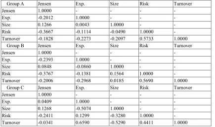
Before performing regression analysis, we tested whether collinearity existed among the explanatory variables because fund variables influence each other. For example, if two or more explanatory variables have highly linear relationships, this is referred to as near multicollinearity. Table 4 indicates that the correlation coefficients were all less than 0.7. Our preliminary view was that high correlations did not exist among the variables.
Table 4. Correlation analysis of relative variables
Group A Jensen Exp. Size Risk Turnover
Jensen 1.0000 - - - -
Exp. -0.2012 1.0000 - - -
Size 0.1266 0.0043 1.0000 - -
Risk -0.3667 -0.1114 -0.0490 1.0000 -
Turnover -0.1828 -0.2273 -0.2097 0.5733 1.0000
Group B Jensen Exp. Size Risk Turnover
Jensen 1.0000 - - - -
Exp. -0.2393 1.0000 - - -
Size 0.0848 -0.0860 1.0000 - -
Risk -0.3767 -0.1381 0.1564 1.0000 -
Turnover -0.2006 -0.2968 0.0185 0.5690 1.0000
Group C Jensen Exp. Size Risk Turnover
Jensen 1.0000 - - - -
Exp. 0.0409 1.0000 - - -
Size 0.1268 -0.5074 1.0000 - -
Risk -0.2411 0.1299 -0.3280 1.0000 -
Turnover -0.0341 0.6590 -0.5290 0.4411 1.0000
Note: We obtained our samples from the TEJ database. The sample data were from January 1, 2001 to December 31, 2012. Group A comprised overall domestic stock fund investors, Group B comprised insured investors, and Group C comprised noninsured investors. Variable definition: Jensen’s alpha represents the excess returns generated by a portfolio. Expense ratio is the sum of management fees (NTD), custodial fees (NTD), guarantee fees (NTD), and other fees (NTD). Fund risk is the annualized standard deviation calculated from the monthly
rate of return over the most recent 12 years. The calculation formula is σi . Fund scale is net assets per
month of each of the funds during the research period. When performing empirical analysis, we derived and used the natural logarithm of the value of each fund’s net assets. The calculation formula for fund turnover rate is the average of the sum of purchase turnover and sales turnover.
Table 5 is the factor table of the coefficients of variation for Group A, B and C. The results indicate that the highest VIF among the individual variables was 1.699. The average VIF was merely 1.3596, indicating that near multicollinearity was not present. The results from the factor table of the coefficients of variation for Group B indicate that the highest VIF among the individual variables was 1.745. The average VIF was merely 1.396, indicating that near multicollinearity was not present. The results from the factor table of the coefficients of variation for Group C indicate that the highest VIF
720 among the individual variables was 2.377. The average VIF was merely 1.7012, indicating that near multicollinearity was not present.
Table 5. The factor table of the coefficients of variation for Group A, B and C.
1/VIF value VIF value
Group A Group B Group C Group A Group B Group C
Jensen 0.794 0.753 0.923 1.259 1.328 1.084
Exp. 0.884 0.813 0.487 1.1312 1.23 2.051
Size 0.933 0.942 0.642 1.072 1.062 1.559
Risk 0.611 0.573 0.697 1.636 1.745 1.435
Turnover 0.589 0.618 0.421 1.699 1.618 2.377
Note: We obtained our samples from the TEJ database. The sample data were from January 1, 2001 to December 31, 2012. Group A comprised overall domestic stock fund investors, Group B comprised insured investors, and Group C comprised noninsured investors. Variable definition: Jensen’s alpha represents the excess returns generated by a portfolio. Expense ratio is the sum of management fees (NTD), custodial fees (NTD), guarantee fees (NTD), and other fees (NTD). Fund risk is the annualized standard deviation calculated from the monthly
rate of return over the most recent 12 years. The calculation formula is σi . Fund scale is net assets per
month of each of the funds during the research period. When performing empirical analysis, we derived and used the natural logarithm of the value of each fund’s net assets. The calculation formula for fund turnover rate is the average of the sum of purchase turnover and sales turnover.
4.2. Quantile regression analysis
In this study, we investigated behavioral differences in Taiwanese domestic equity fund market investors who purchased funds with investment-linked insurance policies and those who directly purchased funds from asset management companies. Regarding quantile regression, cutting quantile values extremely finely facilitates the discovery of comparatively more comprehensive results. Therefore, we selected 10 quantiles to capture the left tails, centers, and right tails of the conditional distributions. We did this to observe the relationships between performance, flows, and other fund characteristics under a variety of conditions.
4.2.1. Relationships Between Fund Inflows, Performance, and Other Fund Operating Characteristics
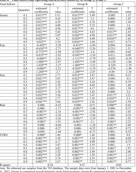
Table 6 indicates that the fund Inflows and performance sensitivity of Group A and Group B present a convex curve relationship. When Inflows were high, the reaction toward performance became strong. Quantiles 0.1 to 0.9 are statistically significant. These results are similar to those of Chevalier and Ellison (1997), Jank and Michael (2013), and Sirri and Tufano (1998). Jank and Michael (2013) found a positive relationship between fund Inflow and performance. In addition, fund Inflows grow as performance is strengthened. In our analysis of the fund Inflows and performance of Group C, the strength of fund Inflows did not significantly react with performance; regardless of the strength of fund Inflows, performance remained the same. Table 6 indicates that the performance and flow sensitivity of Group C were far lower than the sensitivity of Group B. These results are similar to those of Chen et al. (2007), who analyzed the flow and performance sensitivity of insurance company funds and noninsurance company funds.
Table 6 indicates that the fund Inflows and expense ratios of Group B were negatively correlated. Quantiles 0.1 to 0.9 were significant under significant relationships of 5% and 1%. This indicates that expense ratios were low with high subscription rates; that is, investors tended to purchase funds with low expense ratios. This is consistent with the results of Houge and Wellman (2007) and Huang et al. (2007). Houge and Wellman (2007) indicated that when investors begin to be concerned with the expenses of the funds in which they invest, they tend to invest in funds with low expense ratios. Huang et al. (2007) used expense ratio as a control variable in a regression model. The influence of expense ratio reduces the information costs of fund investors. After controlling for expense ratio, high expense ratios lead to reduced fund flows. Relatively low expense ratios attract new investors because of improvements in fund performance. The sensitivity of the relationship between fund flow and performance is increased when performance is excellent. Our analysis of Group C indicated that although fund flow was negatively correlated with expense ratio, this correlation was not statistically significant. This result differs from that of Group B and indicates that insured investors are highly
721 concerned with the expenses of the funds in which they invest and prefer to purchase funds with low expense ratios.
Table 6. Fund Inflows and Operating characteristics sensitivity of Group A, B and C.
Fund Inflows Group A Group B Group C
Quantiles estimated
coefficients
T value
estimated coefficients
T value
estimated coefficients
T value
Jensen 0.1 0.013*** 3.51 0.012*** 3.49 0.005 1.53
0.2 0.017*** 4.43 0.013*** 3.2 0.008- 1.47
0.3 0.015*** 4.29 0.015*** 4.76 0.009- 1.56
0.4 0.015*** 4.88 0.016*** 5.23 0.009- 1.6
0.5 0.017*** 4.94 0.017*** 4.6 0.011- 2.08
0.6 0.021*** 5.02 0.022*** 4.65 0.013** 2.43
0.7 0.025*** 5.07 0.026*** 4.99 0.013** 2.06
0.8 0.029*** 4.2 0.029*** 4.49 0.016** 1.65
0.9 0.025** 2.54 0.036*** 3.68 0.017- 0.73
Exp. 0.1 -0.458** -2.28 -0.415** -2.44 0.094- 0.64
0.2 -0.636*** -2.71 -0.648*** -3.26 0.215- 1.51
0.3 -0.772*** -2.94 -0.792*** -3.6 0.093- 0.69
0.4 -0.835*** -2.83 -0.945*** -3.54 0.011- 0.09
0.5 -0.888** -2.61 -1.111*** -3.79 -0.052- -0.39
0.6 -1.008*** -2.87 -1.095*** -3.49 -0.159- -1.04
0.7 -1.028*** -3.27 -1.004*** -3.23 -0.329- -1.39
0.8 -0.806** -2.51 -0.924*** -3.19 -0.574- -1.49
0.9 -1.204*** -2.7 -1.209*** -2.87 -0.89- -1.34
Size 0.1 0.015*** 2.77 0.014*** 2.87 0.001- 0.23
0.2 0.021*** 3.07 0.022*** 3.67 -0.001- -0.2
0.3 0.025*** 3.42 0.027*** 4.24 0.001- 0.39
0.4 0.027*** 3.39 0.031*** 4.05 0.004- 1.46
0.5 0.029*** 3.17 0.035*** 4.17 0.005- 1.59
0.6 0.032*** 3.38 0.034*** 3.82 0.008- 2.6
0.7 0.032*** 3.56 0.031*** 3.47 0.011** 2.21
0.8 0.026*** 2.77 0.029*** 3.38 0.018** 2.3
0.9 0.041*** 3.04 0.039*** 2.92 0.034** 2.59
Risk 0.1 0.000- -0.42 0.000- -0.51 0.000** 0.42
0.2 0.000- -1.17 -0.001** -2.06 0.000- 0.37
0.3 -0.001** -2.16 -0.001*** -2.92 0.001- 1.03
0.4 -0.001** -2.34 -0.001*** -2.66 0.000- 0.34
0.5 -0.001** -2.42 -0.001** -2.29 0.001- 1.92
0.6 -0.001* -1.91 -0.001** -2.1 0.001* 2.25
0.7 0.000- -0.68 -0.001- -1.28 0.001** 2.08
0.8 0.000- -0.27 0.000- -0.25 0.001** 0.72
0.9 -0.001- -1.44 -0.001- -0.72 0.001- 0.52
TURN 0.1 0.000* 1.86 0.000* 1.66 0.000- 0.8
0.2 0.001*** 3.58 0.001*** 3.58 0.000- 0.09
0.3 0.001*** 4.17 0.001*** 4.09 0.000- 0.75
0.4 0.001*** 3.87 0.001*** 3.55 0.001- 1.9
0.5 0.001*** 4.02 0.001*** 3.51 0.001* 1.97
0.6 0.002*** 3.52 0.002*** 3.49 0.001* 2.06
0.7 0.002*** 3.29 0.002*** 3.59 0.001** 2.13
0.8 0.002*** 2.74 0.001** 2.55 0.002** 2.19
0.9 0.002*** 2.67 0.002** 2.22 0.001** 0.77
R-square 0.24 0.27 0.05
Note: We obtained our samples from the TEJ database. The sample data were from January 1, 2001 to December 31, 2012. Group A comprised overall domestic stock fund investors, Group B comprised insured investors, and
Group C comprised noninsured investors. The variables include Jensen, Exp., Size,,Risk, and Turnover. The
722 The analysis results for Group B indicate that fund Inflows and fund scale were positively correlated. Quantiles 0.1 to 0.9 were significant under significant relationships of 5% and 1%. This indicates that fund Inflow influenced fund scale, and that high subscription rates were associated with strong sensitivity in fund scale. Thus, when actively purchasing, investors preferred to purchase mutual funds with large asset sizes. This result is consistent with the work of Huang et al. (2007) and Jank and Michael (2013). Huang et al. (2007) held that economies of scale increase the visibility of funds, providing service and reducing barriers to investment. This is because when funds are linked with large-scale fund families, they attract an increasing amount of net flows, and the relationship between performance and flow is enhanced. Jank and Michael (2013) found that the scale of a fund family influences the relationship between flow and performance; that is, large-scale fund families are accompanied by high redemption and subscription rates. The results for Group C indicate a positive correlation between fund subscriptions and fund assets. However, only strong asset Inflows had statistical significance, which indicates that investors presented positive subscription relationships only when they preferred large-scale funds. This finding is inconsistent with the results of Group B. However, all of the results indicate that increasing fund Inflows intensified the relationship between fund Inflows and fund performance.
Our analysis of Group B indicates a negative correlation between fund Inflows and fund risk, which indicates that insured investors were risk averse when purchasing funds. However, this was significant only during typical fund Inflows. Our analysis of Group C indicates that fund Inflows and fund risk were negatively correlated. This was statistically significant only at times of strong fund Inflows. In addition, the fund risks of Groups A, B, and C did not change substantially when fund Inflows increased. This is consistent with the results of Fu et al. (2010), who indicated that investors do not give much consideration to risk factors when purchasing or redeeming funds with advertisements because fund advertisement changes investors’ risk attitudes. Our analysis results from Group B indicate a positive relationship between fund Inflow and fund turnover rate. Quantiles 0.1 to 0.9 were statistically significantly consistent with Group A. Group C was statistically significant during strong fund Inflows.
4.2.2. Relationships Between Fund Outflows, Performance, and Other Fund Operating Characteristics
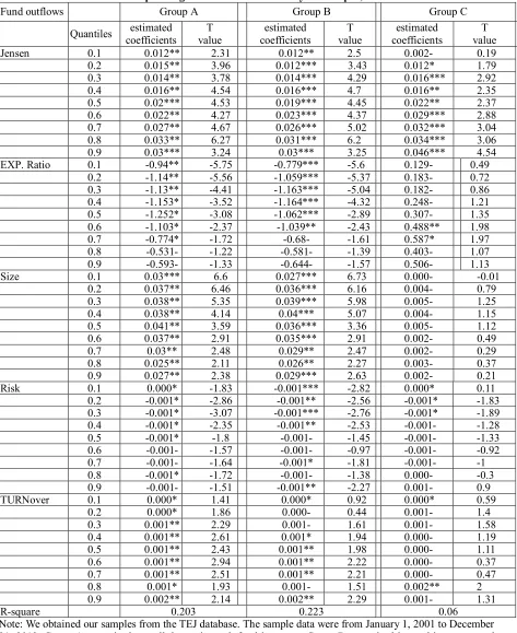
Table 7 indicates that high fund outflows in Group B were associated with strong reactions in performance. Quantiles 0.1 to 0.9 were statistically significant, which means that investors redeemed funds with superior performance. This is the so-called disposition effect. The disposition effect states that stock investors quickly sell the profitable stocks they own and prefer to hold losing stocks for long periods of time. This discovery is consistent with the validation results of Jank and Michael (2013) and Ippolito (1992). Another reason investors redeem funds with superior performance may be to ensure book profit. Thus, they prefer to dispose of assets with capital gains (Kahneman & Tversky, 1979; Frazzini, 2006).
High fund outflows in Group C were associated with strong reactions in performance. Quantiles 0.3 to 0.9 were statistically significant. These results are also consistent with the disposition effect. Regardless of whether mutual funds included investment-linked insurance policies, the redemption behavior of investors was identical. In Group B, fund outflows and expense ratios were negatively correlated. This was statistically significant with weak fund outflows (quantiles 0.1 to 0.4). Fund outflows and expense ratios were positively correlated in Group C. This was statistically significant online in quantile 0.6. These analysis results indicate that insured investors were highly concerned with expense ratios when redeeming funds.
723 during typical fund outflows and strong fund outflows. This indicates that increases in fund turnover rate caused investors to redeem funds actively. The analysis results for Group C indicate that fund outflows were not significant under any of the conditional distributions.
Table 7. Fund outflows and Operating characteristics sensitivity of Group A, B and C.
Fund outflows Group A Group B Group C
Quantiles estimated
coefficients T value
estimated coefficients
T value
estimated coefficients
T value
Jensen 0.1 0.012** 2.31 0.012** 2.5 0.002- 0.19
0.2 0.015** 3.96 0.012*** 3.43 0.012* 1.79
0.3 0.014** 3.78 0.014*** 4.29 0.016*** 2.92
0.4 0.016** 4.54 0.016*** 4.7 0.016** 2.35
0.5 0.02*** 4.53 0.019*** 4.45 0.022** 2.37
0.6 0.022** 4.27 0.023*** 4.37 0.029*** 2.88
0.7 0.027** 4.67 0.026*** 5.02 0.032*** 3.04
0.8 0.033** 6.27 0.031*** 6.2 0.034*** 3.06
0.9 0.03*** 3.24 0.03*** 3.25 0.046*** 4.54
EXP. Ratio 0.1 -0.94** -5.75 -0.779*** -5.6 0.129- 0.49
0.2 -1.14** -5.56 -1.059*** -5.37 0.183- 0.72
0.3 -1.13** -4.41 -1.163*** -5.04 0.182- 0.86
0.4 -1.153* -3.52 -1.164*** -4.32 0.248- 1.21
0.5 -1.252* -3.08 -1.062*** -2.89 0.307- 1.35
0.6 -1.103* -2.37 -1.039** -2.43 0.488** 1.98
0.7 -0.774* -1.72 -0.68- -1.61 0.587* 1.97
0.8 -0.531- -1.22 -0.581- -1.39 0.403- 1.07
0.9 -0.593- -1.33 -0.644- -1.57 0.506- 1.13
Size 0.1 0.03*** 6.6 0.027*** 6.73 0.000- -0.01
0.2 0.037** 6.46 0.036*** 6.16 0.004- 0.79
0.3 0.038** 5.35 0.039*** 5.98 0.005- 1.25
0.4 0.038** 4.14 0.04*** 5.07 0.004- 1.15
0.5 0.041** 3.59 0.036*** 3.36 0.005- 1.12
0.6 0.037** 2.91 0.035*** 2.91 0.002- 0.49
0.7 0.03** 2.48 0.029** 2.47 0.002- 0.29
0.8 0.025** 2.11 0.026** 2.27 0.003- 0.37
0.9 0.027** 2.38 0.029*** 2.63 0.002- 0.21
Risk 0.1 0.000* -1.83 -0.001*** -2.82 0.000* 0.11
0.2 -0.001* -2.86 -0.001** -2.56 -0.001* -1.83
0.3 -0.001* -3.07 -0.001*** -2.76 -0.001* -1.89
0.4 -0.001* -2.35 -0.001** -2.53 -0.001- -1.28
0.5 -0.001* -1.8 -0.001- -1.45 -0.001- -1.33
0.6 -0.001- -1.57 -0.001- -0.97 -0.001- -0.92
0.7 -0.001- -1.64 -0.001* -1.81 -0.001- -1
0.8 -0.001* -1.72 -0.001- -1.38 0.000- -0.3
0.9 -0.001- -1.51 -0.001** -2.27 0.001- 0.9
TURNover 0.1 0.000* 1.41 0.000* 0.92 0.000* 0.59
0.2 0.000* 1.86 0.000- 0.44 0.001- 1.4
0.3 0.001** 2.29 0.001- 1.61 0.001- 1.58
0.4 0.001** 2.61 0.001* 1.94 0.000- 1.19
0.5 0.001** 2.43 0.001** 1.98 0.000- 1.11
0.6 0.001** 2.94 0.001** 2.22 0.000- 0.37
0.7 0.001** 2.51 0.001** 2.21 0.000- 0.47
0.8 0.001* 1.93 0.001- 1.51 0.002** 2
0.9 0.002** 2.14 0.002** 2.29 0.001- 1.31
R-square 0.203 0.223 0.06
Note: We obtained our samples from the TEJ database. The sample data were from January 1, 2001 to December 31, 2012. Group A comprised overall domestic stock fund investors, Group B comprised insured investors, and
Group C comprised noninsured investors. The variables include Jensen, Exp., Size,,Risk, and Turnover. The
724 5. Conclusion and Discussion
In this study, we investigated the Taiwanese domestic equity market and the behavioral differences in insured investors purchasing funds through investment-linked insurance policies and noninsured customers purchasing funds. Because the results for the subscription and redemption behavior of the investors varied, we were unable to explain these behaviors by using only net flows. Therefore, we used a quantile regression model to observe whether performance returns and fund characteristics varied based on the fund Inflows and fund outflows of each group. We also examined whether the behaviors of the investors in each group were consistent with those identified by Chen et al. (2007). Chen et al. stated that the flow and return reactions of funds linked to insurance companies are greater than those of funds not linked to insurance companies regardless of performance quality. In addition, we observed whether the behaviors of the various groups of investors during fund outflows were consistent with the disposition effect proposed by Jank and Michael (2013).
We based this study on whether the domestic equity funds were linked to life insurance companies to divide the investors of funds with investment-linked insurance policies into insured investors and noninsured investors. In addition, we used the TEJ database to analyze the behavior differences caused by the fund flows of mutual funds without investment-linked insurance policies and mutual funds without investment-linked insurance policies in performance returns, fund expense ratios, fund scale, fund risk, and fund turnover rates in the following period. The empirical results indicate that the relationship between performance and flows was stronger among the insured investors than it was among the noninsured investors. This is consistent with the results of Jank and Michael (2013) and Ippolito (1992). In addition, regarding fund characteristics, the relationship between insured investors and fund expense ratios was stronger than it was among the noninsured investors. Fund outflows were consistent with the findings of Huang et al. (2007). After controlling for expense ratio, Huang et al. found that fund flows decreased as expense ratios increased. By contrast, low expense ratios attract new investors because of improvements in performance, which indirectly enhances the sensitivity of the relationship between fund flows and performance when performance is strong.
In this study, we divided the investors of domestic equity funds into insured investors and noninsured investors to analyze the relationships between mutual fund flows, fund performance, and fund characteristics. Although we divided the overall sample into different risk levels and fund scales to analyze the relationships between investment amounts, performance, and characteristics among insured investors, in addition to insured investors, the overall mutual fund market includes a variety of investors from various types of financial institutions. Thus, we were unable to clearly distinguish between the sources of each piece of data. Subsequent researchers can use the channels of other financial institutions when distinguishing groups of investors. Researchers can also cooperate with a number of life insurance companies. Such results could satisfactorily fit the behavior of actual insured investors, which would greatly contribute to both academic and practical fields.
References
Binay, M. (2005). Performance Attribution of US Institutional Investors. Financial Management, 34(2), 127-152.
Chen, C.R., Huang, Y. (2011). Mutual Fund Governance and Performance: A Quantile Regression Analysis of Morningstar's Stewardship Grade. Corporate Governance : An International Review, 19(4), 311-333.
Chen, S, Wu, M., Wang, N. (2008). The Fund Bargain Behavior Analysis of Investment-linked Products: A Study on the Life Insurance Company. Journal of Risk Management, 10(2), 157– 182.
Chevalier, J., Ellison, G. (1999). Are some mutual fund managers better than others? Cross-sectional patterns in behavior and performance. The Journal of Finance, 54(3), 875-899.
Chevalier, J. A. and Ellison, G. (1997). Risk-Taking by Mutual Funds as a Response to Incentives, Journal of Political Economy, 105, 1167-1200.
Chuang, C.C., Kuan, C.M. (2005). Quantile Regression Analysis of the Price-Volume Relationship in Taiwanese and U.S. Stock Markets. Taiwan Economic Review, 33(4), 379–404.
725 Froot, K.A., O'Connell, P.G.J., Seasholes, M. (2001). The portfolio flows of international investors.
Journal of Financial Economics, 59(2), 151-193.
Fu, Y.F., Kang, H.H., and Liu, H. C. (2010). Fund Advertising Effectiveness—Subscription and Redemption. Taiwan Economic Review, 38(3), 459-502.
Goetzmann, W.N., Peles, N. (1997). Cognitive dissonance and mutual fund investors. The Journal of Financial Research, 20(2), 145-158.
Grinblatt, M., Titman, S. (1994). A study of monthly mutual fund returns and performance evaluation techniques. Journal of Financial and Quantitative Analysis, 29(3), 419-419.
Gruber, M.J. (1996). Another puzzle: The growth in actively managed mutual funds. The Journal of Finance, 51(3), 783-810.
Houge, T., Wellman, J. (2007). The Use and Abuse of Mutual Fund Expenses. Journal of Business Ethics, 70(1), 23-23.
Huang, J., Wei, K. D., and Hong, Y. (2007). Participation Costs and the Sensitivity of Fund Flows to Past Performance. The Journal of Finance, 62(3), 1273-1311.
Ippolito, R. A. (1992). Consumer Reaction to Measures of Poor Quality: Evidence from the Mutual Fund Industry. Journal of Law and Economics, 35(1), 45-70.
Ivkovik, Z., Weisbenner, S. (2009). Individual investor mutual fund flows. Journal of Financial Economics,92(2), 223-237.
Jank, S. and Wedow, M. (2013). Purchase and redemption decisions of mutual fund investors and the role of fund families. The European Journal of Finance, 19(2), 127-144.
Jarque, C., Bera, A. (1980). Efficient tests for normality homoscedasticity and serial independence of regression residuals. Econometric Letters, 6, 255–259
Kahneman D. and Tversky, A. (1979). Prospect Theory: An analysis of decision under risk, Econometrica, 47, 263-291.
Koenker, R., and d'Orey, V. (1987). Computing Regression Quantiles, Applied Statistics, 36, 383-393. Lee, J.S., Shen, C.H., Yen, P.H. (2010). Risk States of Funds and Fund Investors’ Disposition Effects:
Application of the Panel Threshold Model. Journal of Management, 27(5), 459-477.
Sirri, E.R., Tufano, P. (1998). Costly search and mutual fund flows. The Journal of Finance, 53(5), 1589-1622.