Privately Efficient Wage Rigidity
Under Diminishing Returns
Bj¨orn Br¨
ugemann
VU University Amsterdam and Tinbergen Institute
June 2014
PRELIMINARY
Abstract
Matching frictions have been shown to reconcile wage rigidity and private effi-ciency in settings with constant marginal returns to labor. A recent line of research has studied the implications of wage rigidity in models with matching frictions and diminishing returns. I show that the allocation of labor is privately inefficient off the equilibrium path in the models used in this line of research, and thus incon-sistent with any theory of wage determination that yields private efficiency. The culprit is rigidity of the wage with respect to firm-level employment. I examine how wage rigidity can be reconciled with private efficiency, focusing on two polar specifications. In the first, wages are rigid with respect to aggregate shocks and flexible with respect to firm-level employment. The labor market responds strongly to aggregate shocks. Yet novel policy implications obtained by this line of research are lost, and thereby shown to be driven by rigidity with respect to firm-level em-ployment. In the second, the wage only adjust when called for by private efficiency, and workers fully appropriate rents in the event of adjustment. Novel policy im-plications obtained in this line of research are restored, including the existence of unemployment in the limit as matching frictions vanish. But fighting this type of rationing unemployment is much easier than in existing models.
Wage rigidity is a perennial topic in macroeconomics. Attempts to explain the cyclical
behavior of employment frequently invoke some kind of wage rigidity. At the same time,
finding a satisfactory microfoundation for rigid wages has long remained elusive. A
long-standing challenge is the Barro critique, aimed at models in which rigid wages result in an
allocation that is privately inefficient for an employer and its employees.1 Responding to
this challenge, Hall (2005) develops a model with matching frictions in which rigid wages
strongly amplify employment fluctuations, without leading to private inefficiencies. Hall
builds on the observation by Howitt (1986) that rigid wages can be consistent with private
efficiency in a labor market with matching frictions. Rogerson and Shimer (2011) argue
that this is in fact the main substantive contribution of search models in the business
cycle context. They observe that matching frictions do not directly help in understanding
cyclical fluctuations in employment, in the sense that they tend to reduce the magnitude
of socially efficient fluctuations. Rather, matching frictions allow for a larger discrepancy
between the socially efficient and privately efficient allocations of labor.
Hall studies a setting with constant marginal returns to labor. A recent line of
re-search initiated by Michaillat (2012) introduces diminishing marginal returns into models
with matching frictions, and finds that the interaction of wage rigidity with diminishing
returns changes the behavior of the labor market qualitatively and delivers several novel
policy implications. Michaillat (2012) shows that in contrast to the model with constant
returns, unemployment remains positive in the limit as matching frictions vanish.
Refer-ring to unemployment in this limit as rationing unemploymenthe finds that the increase
in unemployment in recessions is entirely due to an increase in rationing unemployment,
whereas frictional unemployment actually declines in recessions. Regarding
macroeco-nomic policy, he shows that any policy instrument that acts like a reduction in matching
frictions becomes dramatically less effective at reducing unemployment in recessions.
Im-portantly, with references to the Barro critique and Hall (2005), Michaillat emphasizes
that wages respect private efficiency in his theory.2 Several papers have used a version of
Michaillat’s model to study various macroeconomic and labor-market policies.
Michail-1This critique, developed in Barro (1977, 1979), was originally aimed at a particular class of implicit
contract models.
lat (2014) extends the model by introducing public employment. He shows that the
public-employment multiplier, defined as the effect of an increase in public employment
on total employment, is strongly countercyclical. Landais et al. (2013) analyze optimal
unemployment insurance (UI) over the business cycle in a general matching model. In
their model, optimal UI deviates from the standard Baily-Chetty formula if the level of
labor market tightness is socially inefficient, and if UI has an effect on tightness. In a
version of the model with rigid wages and constant marginal returns, UI has no effect on
tightness and optimal UI is always given by the Baily-Chetty formula. In contrast, with
diminishing returns and rigid wages as in Michaillat (2012), they find that in recessions,
when tightness is inefficiency low, optimal UI is more generous than the Baily-Chetty
formula. Cr´epon et al. (2013) use a version of the model of Landais et al. (2013) to study
the displacement effects of labor market policies.
The first contribution of this paper is to show that the allocation of labor is privately
inefficient off the equilibrium path in the models used in this line of research. This is in
contrast to Hall’s model, in which the allocation of labor is privately efficient both on
and off the equilibrium path. It implies that the theory is inconsistent with any privately
efficient theory of wage determination, including the double auction used by Hall to
characterize wage determination. The culprit is rigidity of the wage with respect to
firm-level employment. In Hall (2005) the wage is rigid with respect to aggregate shocks.
It also does not respond to firm-level employment, but this is natural and does not
interfere with private efficiency in a setting with constant returns. By placing bounds
on exogenous aggregate shocks, Hall (2005) ensures that a constant wage is privately
efficient, avoiding the need to specify how the wage is adjusted in situations in which
this is required to maintain private efficiency. In Michaillat’s (2012) specification the
wage is also rigid with respect to both aggregate shocks and firm-level employment.
Because of diminishing returns, however, a firm can always trigger a situation in which
private efficiency requires a wage reduction via a sufficiently large expansion in hiring.
This cannot be ruled out through a simple restriction on exogenous variables, since the
private inefficiency is triggered by an endogenous choice of firms.
un-avoidable to take a stand on how wages adjust in response to firm-level employment. As
in the case of constant returns, many wage schedules are consistent with private efficiency.
The second contribution of this paper is the analysis of two polar specifications, which
span the range of possibilities for how the wage responds to firm-level employment.
In the first specification, wages are rigid with respect to aggregate shocks and fully
flexible with respect to firm-level employment. I refer to this as the employment-flexible
specification. Wage rigidity with respect to aggregate shocks ensures amplification of
employment fluctuations as in Hall (2005). Thus this specification extends the key
re-sult of Hall (2005) to a setting with diminishing returns: employment fluctuations are
amplified through wage rigidity, without violating private efficiency. At the same time,
I find that the novel policy implications obtained by the line of research initiated by
Michaillat (2012) are lost if this specification is used. Rationing unemployment does not
exist. Policy instruments which act like a reduction in matching frictions retain their
ef-fectiveness to reduce unemployment in recessions. In the context of Landais et al. (2013),
optimal unemployment insurance should not become more generous in recessions. In the
context of Michaillat (2014), the multiplier of government employment is acyclical. By
isolating rigidity with respect to aggregate shocks from rigidity with respect to firm-level
employment, this analysis demonstrates that it is the latter type of rigidity which drives
these policy implications.
The second specification maximizes the extent to which wages are rigid with respect
to firm-level employment while maintaining private efficiency. First, wages do not
re-spond at all as long as this is consistent with private efficiency. Second, if an adjustment
is required, then the wage remains as high as possible, which implies that the workers
fully appropriate rents. Due to the latter feature, I refer to this as the full-appropriation
specification. This specification delivers exactly the same equilibrium as Michaillat’s
specification across values of the aggregate shocks, and also across the type of policies
that have been considered in this line of research. Thus rationing unemployment does
exist, and the novel policy implications derived in this line of research all apply. At
the same time, the policy implications differ substantially if the government fully
but can restore full employment under the full-appropriation specification. Thus fighting
rationing unemployment is much easier in the privately efficient model.
The third contribution of the paper focusses specifically on the existence of rationing
unemployment. The analysis of the full-appropriation specification shows that rationing
unemployment exists in this case, yet full appropriation may appear very restrictive. This
raises the question whether there isanyspecification of technology and wage schedule that
could deliver rationing unemployment without violating private inefficiency and without
invoking full appropriation. I show that the answer is negative: if private efficiency
is required, then full appropriation is both necessary and sufficient for the existence of
rationing unemployment.
1
Model
The model builds on Pissarides (2000, Chapter 1), introducing two modifications. First,
it allows for diminishing marginal returns to labor at the firm level. Second, rather than
assuming that wages are determined through Nash bargaining, wages are given by a
general wage schedule which nests a broad set of bargaining solutions as well as
reduced-form rigid wages. Hall’s (2005) model is obtained as the special case with constant
returns and rigid wages. Michaillat’s general model is dynamic and stochastic. Here I
use a version of the model in which matching and production occur only once. This
version suffices for the purposes of this paper. The analysis immediately carries over to
the dynamic stochastic model, but presenting it in that context would require heavier
notation.
There is a unit mass of ex ante identical firms of unit mass, and a unit mass of workers
per firm. All workers are ex ante identical. Each firm operates a technology described
by the production function g. If a firm employs a mass n of workers at the time of
production, then its output isg(n, a). Herea is the aggregate state of technology. It lies
in [a,a¯] ⊂ (0,+∞). The function g is differentiable and weakly concave in n, satisfies
g(0, a) = 0 for all a ∈ [a,¯a], and is strictly increasing in both arguments. Workers that
of workers is given by expected consumption. Firms maximize expected profits.
The model has two stages. In the first stage, each firm decides how many workers
to hire. In the second stage, wages and employment are determined in each firm, and
production takes place.
For simplicity, I assume that all workers are initially unmatched.3 Firms can recruit
workers by opening vacancies. I specify the matching technology through two functions
q(θ) and f(θ), where θ denotes labor-market tightness, q(θ) is the probability that a
vacancy is filled, andf(θ) is the probability than an unemployed worker finds a job. This
specification can be derived from a constant-returns-to-scale matching function, with
tightness defined as the vacancy-unemployment ratio, and in this case the two functions
are linked through the restriction f(θ) =θq(θ). I do not impose this restriction in what
follows. This turns out to be useful in Section 4. The function q : [0,+∞) → [0,1]
is strictly decreasing, f : [0,+∞) → [0,1] is strictly increasing, and both functions are
continuous.
To hiren1 workers, a firm must open qn(θ1) vacancies. Here the subscript ofn1indicates
that hiring is chosen in the first stage. The firm incurs a cost c·a per vacancy. Here
c ∈ [0,+∞) is the parameter governing the cost of recruiting. Vanishing matching
frictions are modeled by letting c converge to zero. To ensure that matching frictions
indeed vanish asc goes to zero, the matching technology satisfies limθ→+∞f(θ) = 1.
Each possible level of hiring n1 ∈ [0,+∞) by a firm in the first stage leads to a
subgame in the second stage, indexed byn1, in which the wage and the employment level
in the firm are determined. This subgame is not modeled explicitly. Instead, its outcome
is described as follows. The wage is determined by a general wage schedulew(n, a), where
n is the employment level at the firm at the time of production. The wage schedule is
differentiable innand non-negative. As discussed by Michaillat, this specification nests a
3Allowing for an initial positive level of employment does not change any of the results derived in
broad set of bargaining solutions as well as reduced-form rigid wages. Define the function
Π(n, a)≡g(n, a)−w(n, a)n. (1)
It gives the ex-post profits of a firm with employment n, defined as profits excluding
recruiting costs sunk in the first stage. Employment in subgame n1 is assumed to be
profit-maximizing. Let
N2(n1)≡arg max
n∈[0,n1]Π(n, a) (2)
denote the set of profit-maximizing employment levels. For simplicity, it is assumed that
in case of indifference a firm chooses the highest profit-maximizing employment level,
that is,n2(n1) = maxN2(n1).
I now define an equilibrium. In doing so, I make explicit that employment levels in all
subgames are equilibrium objects. I restrict attention to symmetric equilibria in which
hiring in the first stage and the outcome in all subgames are the same across firms.
Definition 1 A level of labor market tightness θ, a first-stage employment level n1, and second-stage employment levels{n2(n1)}n1∈[0,+∞) constitute an equilibriumfor given a∈
[a,¯a] if
1.
n1 ∈arg max
n∈[0,+∞)
Π (n2(n), a)− c·a
q(θ)n
. (3)
2. n2(n1) = maxN2(n1) for all n1 ∈[0,+∞).
3. The first-stage employment level n1 and labor market tightness satisfy
n1 =f(θ). (4)
Condition 1 requires that firms maximize ex-ante profits in the first stage. Condition
2 specifies the outcome of subgame n1 according to the discussion above. Condition 3
requires that the number of workers n1 hired by firms for a given level of θ is consistent
2
Private Efficiency
The allocation of labor in subgame n1 is privately efficient if the firm and its hires
exploit all opportunities for mutual improvement. In the present model, the privately
efficient allocation is easy to determine. Since the firm maximizes expected profits while
workers’ utility is given by expected consumption, it is clear that private efficiency requires
maximization of output. Because the production functiong(n, a) is strictly increasing in
n and since unemployed workers produce zero, private efficiency requires that all hires
are employed at the time of production. Hence, for this model, we can define private
efficiency in subgame n1 as follows.
Definition 2 An allocation of laborn2(n1)in subgamen1isprivately efficientifn2(n1) = n1.
Any theory of wage determination that generates privately efficient outcomes would imply
that the allocation of labor is privately efficient in all subgames n1 ∈ [0,+∞). The
following lemma provides a simple characterization of private efficiency in all subgames
in terms of the function Π(n, a).
Lemma 1 Letθ, n1, and{n2(n1)}n1∈[0,+∞) be an equilibrium for givena. The allocation
of labor is privately efficient in all subgames n1 ∈[0,+∞)if and only if Π(n, a) is weakly
increasing in n.
Proof: Suppose that Π(n, a) is weakly increasing. Consider subgame n1. Then n1 ∈
N2(n1), and consequently n2(n1) = n1. Conversely, suppose that Π(n, a) is not weakly
increasing. Then there exist two employment levels nH and nL such that nH > nL and
Π(nH, a)<Π(nL, a). Thus the allocation of labor is privately inefficient in subgamenH,
contradicting private efficiency in all subgames.
In a setting with constant marginal returns to labor, Hall (2005) obtains a rigid wage
schedule as an equilibrium outcome by characterizing wage determination in terms of a
double auction. In the auction, both the worker and the firm simultaneously propose
wages wA and wB, respectively. If wA ≤wB, trade occurs at the wage w =κwA+ (1−
lies between the reservation wage of the worker and the reservation wage of the firm is
a Nash equilibrium. Consequently, with constant returns g(n, a) = a·n any wage in
the interval [0, a] is an equilibrium. As a consequence, the wage need not adjust one
for one with changes in a. Even a constant wage is possible, as long as it does not lie
below the lowest state of technology a. It is the indeterminacy of the double auction
which permits wage rigidity to be an equilibrium outcome. The auction permits many
alternative equilibrium wage patterns, and Hall’s theory does not aim to explain why a
rigid wage pattern is chosen.
Hall’s theory is easily generalized to a setting with diminishing marginal returns by
building on the theory of intra-firm bargaining developed by Stole and Zwiebel (1996).
Stole and Zwiebel model pairwise negotiations through the Nash bargaining solution. To
obtain a theory of intra-firm bargaining, they define a notion of stability. The key feature
of this notion is that a breakdown of negotiations between the firm and a given worker is
followed by a renegotiation with all remaining workers. It is straightforward to adapt this
approach by replacing the Nash bargaining solution with the double auction, retaining
the notion of stability proposed by Stole and Zwiebel.
Consider a pairwise negotiation between a worker and a firm when the level of
em-ployment isn. In the event of breakdown the worker receives zero, while the firm receives
gn(n, a)−nwn(n, a) where the subscriptnindicates the partial derivative with respect to
firm-level employment. To understand this payoff of the firm, notice that if the pairwise
negotiation fails, the firm not only loses the marginal product gn(n, a), but its wage
pay-ments to the remaining workers change by−nwn(n, a). Consequently, the bargaining set
in the pairwise negotiation is [0, gn(n, a)−nwn(n, a)]. According to the Nash
bargain-ing solution the wage w(n, a) is the midpoint of this interval. This yields a differential
equation with a unique solution. Replacing the Nash bargaining solution with the double
auction, any wage in the bargaining set is a Nash equilibrium in the pairwise negotiation.
Thus w(n, a) must satisfy w(n, a)≥0 and the differential inequality
This differential inequality can also be written as Πn(n, a)≥0. This result is summarized
in the following proposition.
Proposition 1 The bargaining outcome given by the functions w(n, a) and Π(n, a) is a Nash equilibrium of the double auction at every level of employment n and stable in the
sense of Stole and Zwiebel (1996) if and only if w(n, a) is non-negative and Π(n, a) is
weakly increasing in n.
In light of Lemma 1, an immediate corollary is that the wage schedule w(n, a) gives rise
to a privately efficient allocation in all subgames if and only if the bargaining outcome
described by the functionsw(n, a) and Π(n, a) is a Nash equilibrium of the double auction
at every level of employment and stable in the sense of Stole and Zwiebel.
3
Private Inefficiency in Michaillat’s Theory
In this section I introduce the specification with diminishing marginal returns to labor
and rigid wages. I examine the private efficiency properties of equilibrium, and observe
that the allocation of labor is privately inefficient in a set of subgames off the equilibrium
path.
The production function is
g(n, a) = anα (5)
with α∈(0,1) and the wage schedule is
w(n, a) =ωaγ (6)
with ω ∈ (0,+∞) and γ ∈ [0,1). Since γ < 1, the wage is rigid in the sense that it
does not respond proportionally to changes in the aggregate state of technology. This is
the type of rigidity considered by Hall (2005). Importantly, wage schedule (6) exhibits
a second type of rigidity: the wage does not respond to the number of workers recruited
by the firm. This is natural in an environment with constant marginal returns to labor.
to private inefficiency in some subgames. From now on, I refer to equations (5)-(6) as
Michaillat’s specification. It implies the ex-post profit function
Π(n, a) =anα−ωaγ. (7)
Solving the maximization problem in equation (2) yields
n2(n1) = min{n1, nR(a)} (8)
where
nR(a)≡α
ω
11
−α
a11−−γα. (9)
Here nR(a) is the maximal mass of workers the firm is willing to retain after recruiting costs are sunk. Thus employment is given by nR(a) in any subgame with n
1 ≥ nR(a).
The hiring-stage objective function specified in equation (3) is then given by
anα−ωaγn− c·a
q(θ)n, ifn ≤nR(a),
a(nR(a))α−ωaγnR(a)−qc(·θa)n, ifn > nR(a).
(10)
This objective is maximized by
n1 =nd(θ, a, c)≡
[nR(a)]−(1−α)+ c
αq(θ)
−11
−α
. (11)
As long as c
q(θ) is strictly positive, hiring n
d(θ, a, c) is strictly below nR(a). That is, the
firm is recruiting fewer workers than it is willing to retain after recruiting costs are sunk.
Substituting the optimal level of hiring nd(θ, a, c) into equation (4) yields a condition that implicitly determines equilibrium tightness
f(θ) =nd(θ, a, c). (12)
It is easy to check that this equation has a unique solution.
Michaillat studies the behavior of equilibrium employment as matching frictions
state of technology is sufficiently low.
Definition 3 Given a ∈ [a,¯a], suppose that n(a,c) is an equilibrium level of employ-ment for each c ∈ (0,+∞). Then {n(a, c)}c∈(0,+∞) exhibits rationing unemployment if
limc→0+n(a, c)<1.
The concept of rationing unemployment involves the thought experiment of what would
happen to unemployment as matching frictions vanish. Thus it is defined for a collection
of equilibria {n(a, c)}c∈(0,+∞), one equilibrium for each strictly positive level of the
re-cruiting costc. Zero recruiting cost are excluded here, so the limit taken in the definition
is a righthand limit. This allows for the possibility of a discontinuity at c = 0, that is,
there can be rationing unemployment even if c= 0 implies full employment.
Let θ(a, c) denote the solution to equation (12) for given values of a ∈[a,a¯] and c∈
(0,+∞). Then the corresponding equilibrium level of employment along the equilibrium
path is n(a, c) ≡ f(θ(a, c)). Michaillat establishes the following result: if nR(a) < 1,
then limc→0+n(a, c) = nR(a); if nR(a) ≥ 1, then limc→0+n(a, c) = 1.4 Thus rationing
unemployment exists if and only if nR(a)<1. If the firm does not want to retain a unit
mass of workers after recruiting costs are sunk, then full employment cannot be attained
even asc converges to zero.
Next, I examine the private efficiency properties of equilibrium. Consider the
equi-librium for given values of a and c. Equation (11) implies that n1 ≤ nR(a). Inspecting
equation (8), this means that the constraint n ≤ n1 is binding in subgame n1. Thus
n2(n1) = n1, hence the allocation of labor is privately efficient along the equilibrium
path.5
Equation (8) also implies that the allocation of labor is notprivately efficient in any
subgame n1 in which n1 > nR(a). In any such subgame, a firm has recruited more
workers than it is willing to employ given wage schedule (6). In this situation, it would
be privately efficient for the wage to adjust such that is optimal for the firm to employ
4This is Proposition 4 in Michaillat (2012). The statement given here is slightly more compact, as
Michaillat definesnR(a) in the proposition. The thresholdaR used by Michaillat in his statement of the
proposition is defined implicitly bynR(aR) = 1.
5In his Definition 2, Michaillat (2012) defines when a wage process is privately efficient. This definition
alln1 hires.
The result that the allocation of labor isnotprivately efficient in some subgames also
follows immediately from Lemma 1 in conjunction with the fact that Π(n, a) is strictly
decreasing for n ≥ nR(a). From Proposition 1 it also follows that wage schedule (6)
cannot be obtained as the equilibrium of the model of wage determination that combines
the double auction used by Hall (2005) with intra-firm bargaining as in Stole and Zwiebel
(1996).
It is useful to contrast this result with the case of constant returns, obtained by setting
α= 1. With constant returns and wage schedule (6), the allocation of labor is privately
efficient in subgamen1 ifω≤a1−γ. This condition does not depend onn1, thus condition
ω ≤ a1−γ ensures private efficiency in all subgames n
1 ∈[0,+∞). Furthermore, private
efficiency across all states of aggregate technology can be ensured by assuming that
ω ≤a1−γ. (13)
This result is a simple generalization of Hall’s (2005) Proposition to the case in which
the wage is partially responsive to the aggregate state of technology. If condition (13) is
assumed, then there is no need to specify how the wage is adjusted in situations in which
the wage schedule (6) would generate private inefficiency, because such situations arise
neither on nor off the equilibrium path.
In contrast, with diminishing returns, wage schedule (6) implies that there are always
subgames in which the allocation of labor is privately inefficient, irrespective of the level
of technologya. Thus there is no simple restriction on exogenous variables which ensures
private efficiency in all subgames, short of assumingω = 0. The reason for this difference
is that private inefficiency can be triggered via the endogenous choice of employment by
the firm. With diminishing returns, private efficiency dictates that the wage schedule
w(n, a) cannot be fully independent of firm-level employment. To reconcile wage rigidity
and private efficiency, it is thus unavoidable to take a stand on how wages adjust in
response to firm-level employment. Now, private efficiency only requires that Π(n, a) is
outcomes, the next two sections study the implications of two polar specifications which
span the range of possibilities.
4
Employment-Flexible Wage Schedule
As discussed in Section 3, wage schedule (6) exhibits two types of rigidity. First, the wage
does not respond proportionally to changes in technology. Second, the wage is also rigid
in that it does not respond to the mass of workers recruited by the firm. The strength
of the first type of rigidity is indexed by the parameter γ. In contrast, the second type
of rigidity is absolute. Symmetrically to the first type of rigidity, one can parametrize
the strength of the second rigidity by letting the wage respond to firm-level employment
with a constant elasticity. This leads to the more general wage schedule
w(n, a) = ωaγnφ, (14)
with γ ∈ [0,1), ω > 0, and φ ∈ (−∞,+∞). Here the parameter φ controls the second
type of rigidity, and Michaillat’s wage schedule (6) is nested as the special case φ = 0.
Now consider the specification consisting of production function (5) and wage schedule
(14). As discussed in Section 3, withφ= 0 this specification necessarily generates private
inefficiency off the equilibrium path. This raises the question for what values ofφ, if any,
wage schedule (14) can be consistent with private efficiency off the equilibrium path. It is
easy to see that there is only one such value, namelyφ =α−1.6 In other words, subject to
the restriction that the wage responds to firm-level employment with a constant elasticity,
private efficiency off the equilibrium path requires that the wage schedule takes the form
w(n, a) =ωaγnα−1. (15)
6LetnR(a, φ)≡[α/(ω(1 +φ))]1/(1+φ−α)a(1−γ)/(1+φ−α). Ifφ > α−1, then Π(n, a) =anα−ωaγn1+φ
is strictly decreasing innon
nR(a, φ),+∞
, hence the allocation of labor is privately inefficient in any subgamen1 withn1> nR(a, φ). Ifφ < α−1, then Π(n, a) is strictly decreasing on 0, nR(a, φ), hence
For private efficiency across all states of aggregate technology, condition (13) is necessary
and sufficient. Thus the restriction on exogenous variables is exactly the same as in the
case of constant returns, and in this sense wage schedule (15) is a natural generalization of
Hall’s theory to a setting with diminishing marginal returns. For what follows, I assume
that condition (13) holds.
Ex-post profits are given by
Π(n, a) = [a−ωaγ]nα
and thus weakly increasing inn for all levels ofa. Thusn2(n1) =n1 for alln1 ∈[0,+∞),
ensuring private efficiency. A firm then chooses hiring n1 to maximize ex-ante profits
[a−ωaγ]nα− c·a
q(θ)n.
This yields
n1 =nd(θ, a, c)≡
q(θ)
c α
1−ωaγ−1
11
−α
It follows immediately that here the collection of unique equilibria {n(a, c)}c∈(0,+∞) does
not exhibit rationing unemployment, irrespective of the aggregate state of technology.
Consider the equilibrium as cconverges to zero. For rationing unemployment to exist, it
must be that equilibrium labor market tightness θ(a, c) does not diverge to infinity. But
then q(θ(ca,c)) converges to zero, which implies that labor demandnd(θ(a, c), a, c) converges to infinity, which is inconsistent with equilibrium.
Is it plausible that wages could be rigid with respect to aggregate shocks but flexible
with respect to firm-level employment? Hall’s theory does not speak to this question,
since it does not explain why rigidity with respect to aggregate shocks is chosen among
the wide variety of privately efficient wage schedules. Hall offers the interpretation of a
wage norm, and it is conceivable that the strength and applicability of wage norms differs
across different reasons for wage changes. Most recent empirical work on wage rigidity
has focussed on the response of wages to aggregate shocks. Less is known about how
Bewley (1999) supports both types of rigidity. However, as discussed by Hall, Bewley’s
work is aimed at explaining outcomes that are privately inefficient when viewed through
the lens of standard theory. If this evidence accurately portrays the operation of the
labor market, then this does not support a theory of wage rigidity insisting on private
efficiency, and would instead call for a theory explaining privately inefficient outcomes.
In the remainder of this section I analyze further implications of the
employment-flexible specification. Recall that in Section 1 I did not impose a restriction linking the
functionsf(θ) and q(θ). Usually these functions are derived from a
constant-returns-to-scale matching function, defining tightnessθ as the vacancy-unemployment ratio. In this
case the two functions are linked through the restriction f(θ) =θq(θ). Here I adopt the
more general specification
f(θ) = θq(θ)
(1−s)θq(θ) +s (16)
where s ∈[0,1] is a parameter. Furthermore, I assume that q(θ) has the Cobb-Douglas
functional form
q(θ) = min
µθ−η,1
withµ∈(0,+∞) andη∈(0,1). The usual casef(θ) =θq(θ) is obtained by settings = 1.
The benefit of the more general specification is that with s interpreted as the exogenous
separation rate, the equations determining equilibrium tightness and employment are
exactly the same as the equations determining steady-state tightness and employment
in the dynamic version of the model with a Cobb-Douglas matching function.7 In this
way the one-shot model can be used to emulate the response of the steady-state of the
dynamic model.
For a given function Π, induced by one of the two wage schedules (6) and (15), the
labor demand schedule nd(θ, a, c) is defined implicitly by the condition
Πn(nd(θ, a, c), a) =
c·a
q(θ). (17)
7In the equilibrium of the one-shot model we have n = f(θ). Substituting this relationship into
Define the labor supply schedule asns(θ)≡f(θ). Then equilibrium tightness must satisfy
the condition
ns(θ) =nd(θ, a, c). (18)
All of the implications studied below are driven by the properties of labor demand and
labor supply elasticities. Thus it is useful to derive these elasticities before considering
specific implications. Letǫs
θ denote the elasticity of labor supply with respect to tightness.
Differentiating equation (16), it is given by
ǫsθ = (1−η) [1−(1−s)n]. (19)
In the standard one-shot case with s= 1, this elasticity reduces to 1−η, which is simply
the elasticity of the job-finding probability with respect to tightness. In the steady-state
interpretation of the model with s representing the exogenous separation rate, the labor
supply elasticity is lower when employment is high. This is because fewer workers are
available for matching, implying that a given percentage increase in tightness delivers
only a smaller percentage increase in employment.
Differentiating equation (17), the elasticity of labor demand with respect to tightness
is
ǫdθ =η
ǫΠn
n
−1
(20)
whereǫΠn
n denotes the elasticity of marginal ex-post profits with respect to employment.
If η is high, then a decrease in tightness has a strong effect on the probability that a
vacancy is filled, and thereby on the cost of hiring a worker, resulting in a stronger
increase in labor demand. If marginal ex-post profits decline quickly as employment
expands, this dampens the increase in employment.
The difference between the wage schedules (6) and (15) manifest itself in the
elas-ticity ǫΠn
n . First, consider the employment-flexible schedule (15). Here Πn(n, a) =
α[a − ωaγ]n−(1−α). Thus the elasticity is ǫΠn
n = −(1 −α). Here both the marginal
product of labor and ex-post marginal labor cost respond to employment with the same
Michaillat’s wage schedule (6). Here Πn(n, a) = αan−(1−α)−ωaγ. Thus
ǫΠn
n =−(1−α)
1 1− ωaγ
aαnα−1 .
Notice that ǫΠnn
is high if ωa γ
aαnα−1 is high, that is, if the wage is high relative to the marginal product of labor. With wage schedule (15), an increase in employment reduces
marginal ex-post profits, but this reduction is muted by the fact that the marginal wage
bill also declines. This muting effect is not present under wage schedule (6), since the
wage remains constant as employment increases. Thus marginal ex-post profits are more
responsive to employment, the more so the higher is the level of the wage relative to the
marginal product of labor. Michaillat shows that ǫΠnn
evaluated at the equilibrium level
of employment is decreasing in a. The reason for this is as follows. In equilibrium, the
marginal product of labor must cover two types of marginal costs of labor: the wage and
the hiring cost c·a
q(θ). As a increases, the hiring cost increases faster than the wage, both
becauseq(θ) declines as the labor market tightens, and because of the direct proportional
effect of a. Consequently, the marginal product of labor grows faster than the wage, so
that the ratio ωaγ
aαnα−1 declines. Thus
ǫΠnn
is high in recessions induced by a low state
of aggregate technology, making labor demand unresponsive to changes in labor market
tightness. For exactly the same reasons, a recession induced by an exogenous increase in
ω is also associated with a high ratio ωaγ
aαnα−1, and thus a high elasticity
ǫΠnn
. Generating
a recession through high ω is not substantially different from generating a recession
through a low level of aggregate technology, since what matters in the model is the level
of technology relative to the level of the wage.
4.1
Elasticity of Employment with Respect to Aggregate
Tech-nology
The main finding of Hall (2005) is that privately efficient wage rigidity can strongly
amplify the response of the economy to changes in the aggregate state of technology.
The elasticity of equilibrium employment with respect to the state of technology a is
ǫna =ǫda· ǫ
s θ
ǫs θ+|ǫdθ|
.
Here the first termǫda measures the shift in labor demand induced by a change in a. The second term measures the slope of labor supply relative to labor demand, and determines
how the shift in labor demand translates into a shift in equilibrium employment. The
labor demand shift is given by ǫd a =
ǫΠn
a −1
·ǫΠnn
−1
. Substituting this elasticity and
the labor supply and demand elasticities from equations (19) and (20) yields
ǫna|a=1 =
(1−α) + η
(1−η)[1−(1−s)n]
−1
ω
1−ω(1−γ).
This formula includes the case of constant marginal returns for α = 1. Diminishing
returns attenuate the response of employment to a technology change by making labor
demand steeper. As firms expand employment in response to an improvement in
tech-nology, they run into diminishing marginal returns, and this dampens the response of
re-cruitment. Quantitatively, however, this dampening is not severe for standard parameter
values, since labor supply remains much stepper than labor demand. Using Michaillat’s
(2012) calibration, the elasticity is only 2% lower compared to the case of constant
re-turns.8 In this sense, the amplification of changes in aggregate technology found by Hall
(2005) remains intact if wage schedule (15) is used in the case of diminishing returns.
What matters here is rigidity of the wage with respect to aggregate shocks, and rigidity
of the wage with respect to firm-level employment is not needed. Thus specification (15)
provides a natural generalization of Hall’s findings to a setting with diminishing marginal
returns, reconciling amplification of aggregate shocks through wage rigidity with private
efficiency.
8Only the term in square brackets is affected by α, so only the parameters and variables in this
term are relevant. In Michaillat’s calibration they take the valuesη = 0.5,s= 0.0095, α= 0.666, and
4.2
Elasticity of Tightness with Respect to Recruiting Costs
Michaillat shows that in his model labor market tightness, and thus unemployment,
respond less elastically to changes in the recruiting cost c in recessions. This implies
that any policy instrument that acts like a reduction in the recruiting cost becomes
less effective at reducing unemployment in recessions. Michaillat demonstrates that this
property is quantitatively very important in a calibrated version of the model. I will now
show that this property does not apply to the employment-flexible specification.
In Michaillat’s model a recession corresponds to a low value of the aggregate state
of technology in a. Let ǫθc(a) denote the elasticity of tightness with respect to the re-cruiting costc, with the potential dependence on the state of aggregate technology made
explicit. Michaillat shows thatǫθc(a)
is strictly increasing in afor his specification.9 He
also demonstrates that this property is unique to the specification with rationing
unem-ployment, in the sense that it does not hold for any of the three other specifications of
production function and wage schedule he studies. Michaillat considers two specifications
with flexible wages, namely constant marginal returns to labor combined with Nash
bar-gaining, and diminishing marginal returns to labor combined with intra-firm bargaining
as in Stole and Zwiebel (1996). The two elasticities are always zero for both specifications,
and thus trivially independent of a. The third specification combines constant marginal
returns with the rigid wage schedule (6). This is the specification that corresponds to
Hall (2005). Here the two elasticities are non-zero but do not vary with a.
I will now contrast the behavior of ǫθc(a)
for Michaillat’s wage schedule (6) and the
employment-flexible wage schedule (15). Implicitly differentiating labor-market
equilib-rium condition (18) yields
ǫθc(a) =ǫdc(a)· 1
ǫsθ(a) +|ǫdθ(a)|. (21) The first term ǫdc(a) captures the shift in labor demand induced by a change in the recruiting cost. The second term translates this into a change in equilibrium tightness,
9This is Proposition 6 in Michaillat (2012). The proposition also considers the elasticity of
unemploy-ment with respect to recruiting costs. I focus on ǫθc(a)
depending on the elasticities of labor supply and labor demand. Equation (17) implies
that the labor demand shift is ǫdc(a) =
ǫΠn
n (a)
−1
. A decrease in c reduces the cost of
hiring a worker and leads to an expansion of labor demand, but this expansion is muted
if marginal ex-post profits decline quickly in firm-level employment. This elasticity is
identical to the labor demand elasticity ǫd
θ(a), except that the latter also depends on the
elasticity η because a change in tightness only affects hiring costs to the extent that it
affects the vacancy-filling probability.
Substituting ǫdc(a) and the elasticities of labor demand and labor supply derived in equations (19)–(20) into equation (21) yields
ǫθc(a)
=
η+ǫΠnn(a)
u(a)(1−η) −1
(22)
where u(a)≡1−(1−s)n(a) measures the level of unemployment after production and
exogenous separations have occurred, using the steady-state interpretation of the model.
Since both demand elasticities ǫd
c(a) and ǫdθ(a) are inversely proportional to ǫΠnn(a), the
term ǫΠn
n (a) multiplies the labor supply elasticity in this formula.
To parse this formula, first consider the case of constant marginal returns to
la-bor, which imply that marginal ex-posts profits do not depend on employment, so that
ǫΠn
n (a) = 0, and the elasticity reduces to
ǫθc(a)
= η−1. In this case the first-order
con-dition (17) does not depend on the level of employment, so restoring this concon-dition after
a reduction in c requires that tightness increases to keep the right-hand side c·a q(θ)
con-stant. This adjustment is smaller if the vacancy-filling probability is more responsive to
tightness.
Diminishing returns to labor introduce the additional term ǫΠnn(a)
u(a)(1 −η) in
the formula for ǫθc(a)
. Thus diminishing returns dampen the response of tightness to
a reduction in c. The reason is that now an increase in employment can contribute to
restoring first-order condition (17). The strength of this effect depends on two factors.
First, the responsiveness of labor supply to an increase in tightness. This factor is
re-sponsible for the termu(a)(1−η). Second, the responsiveness of marginal ex-post profits
to an increase in employment ǫΠn
Michaillat’s analysis is concerned with how the elasticity ǫθc(a)
varies with technology
a. It is clear from equation (22) thatǫθc(a)
can depend onaonly through the elasticity of
marginal ex-post profits ǫΠnn(a)
and throughu(a). I will ignore the dependence through
u(a) for now and return to it below. As discussed above, the elasticity ǫΠnn(a)
depends
on the wage schedule. With the employment-flexible wage schedule, this elasticity is
given by 1−α and thus independent of a. In contrast, with Michaillat’s wage schedule
(6), a recession induced by low a is associated with a high elasticity ǫΠnn(a)
, which in
turn implies that ǫθc(a)
is low. In such a recession, a reduction in c has little effect on
employment, because even a small increase in employment leads to a strong decline in
marginal profits, since wages are unresponsive to an expansion of employment, and since
the level of the wage is relatively high.
This comparison with the employment-flexible wage schedule (15) highlights that
this result is intimately related to the fact that the wage is rigid with respect to
firm-level employment. If wages are rigid only with respect to aggregate technology, then a
reduction incis equally effective in reducing unemployment in both booms and recessions.
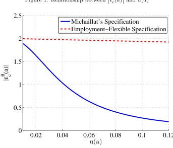
So far I have ignored the dependence ofǫθc(a)
onathroughu(a). In recessionsu(a) is
high, which increases the labor supply elasticity and thus reduces ǫθc(a)
. Quantitatively,
however, the strength of this mechanism is negligible. Figure 1 plots the relationship
between ǫθc(a)
and u(a) traced out by varying the level of a for both wage schedules
under Michaillat’s calibration.10 Unemployment u(a) is on the horizontal axis, and the
elasticity ǫθc(a)
is on the vertical axis. The solid line represents this relationship for
Michaillat’s wage schedule (6), replicating Figure 2 in Michaillat (2012). Asa increases,
u(a) decreases and ǫθc(a)
increases, traveling along the solid line in a northwestern
direction. The dashed line shows the corresponding relationship for wage schedule (15).
This relationship is also negative, reflecting the direct effect thatu(a) has on ǫθc(a)
. Yet
quantitatively the decline in ǫθc(a)
is negligible as unemployment varies from 0.01 to
10The parameter values areδ= 0.999,s= 0.0095,µ= 0.233,η= 0.5,c= 0.215, andα= 0.666. Other
Figure 1: Relationship between ǫθc(a)
and u(a)
0.02
0.04
0.06
0.08
0.1
0.12
0
0.5
1
1.5
2
2.5
u(a)
|
ε
cθ
(a)|
Michaillat’s Specification
Employment−Flexible Specification
0.12. Thus the dramatic decline ofǫθc(a)
obtained for wage schedule (6) is driven by the
effect of a through ǫΠn
n (a).
4.3
Countercyclicality of the Public-Employment Multiplier
Michaillat (2014) introduces public employment into the model of Michaillat (2012).
The government participates in the matching process in exactly the same way as private
firms. The level of public employment g is treated as an exogenous variables. The mass
of vacancies posted by the government adjusts endogenously to reach this level of public
employment. Total labor demand is then
ntd(θ, ω, g) =nd(θ, ω) +g.
Herend(θ, ω) denotes the labor demand of the private sector implicitly defined by
notation, and instead make the dependence onω explicit, since Michaillat (2014) models
recessions as situations with high ω.
Let ǫtd
θ (ω) denote the elasticity of total labor demand with respect to tightness. It is
given by ǫtdθ (ω) = (1 +ζ)−1ǫd
θ(ω), where ζ = g
nd denotes the ratio of public and private
employment and is assumed to be independent of ω.
The labor market clearing condition is now
ns(θ) =ntd(θ, ω, g).
Differentiating with respect to g, the total derivative of total employment with respect
tog is
dn
dg(ω) = 1−
1 + ǫ
s θ(ω)
|ǫtd θ (ω)|
−1
.
Here the one captures the direct effect, while the second term is the crowding out effect.
The latter is a horse race between the labor supply elasticity and the labor demand
elasticity. An increase in g increases labor market tightness. If labor supply is highly
responsive to tightness, then the increase inθ needed to restore labor market equilibrium
is small, and so is the crowding out effect. If the labor demand elasticity is high, then
the increase inθ has a strong negative effect on private labor demand, and crowding out
is strong.
Substituting the labor supply and labor demand elasticities from equations (19) and
(19) yields
dn
dg(ω) = 1−
1 + (1 +ζ)η(1−η)u(ω) ǫΠn(ω)
−1
. (23)
where u(ω) ≡ 1−(1−s)n(ω) denotes unemployment after production and exogenous
separations. Michaillat shows that the public-employment multiplier dn
dg(ω) is increasing
in ω. He concludes that the public-employment multiplier is large in recessions because
crowding out is small. From equation (23), it is clear thatωcan affect the multiplier only
through the elasticity ǫΠnn(ω)
and through u(ω). As discussed in Section 4.2, the latter
effect is negligible. Thus any important effect of ω on the multiplier must act through
the elasticity
ǫΠnn(ω)
the mechanism generating this effect is the same as in Section 4.2. With wage schedule
(6), in recessions wages are more important relative to hiring costs as a component of the
total marginal cost of labor. Since wages are unresponsive to firm-level employment, this
implies a larger absolute value ofǫΠnn(ω)
in recession. In contrast, with the
employment-flexible wage schedule (15) this mechanism is absent. The wage is not rigid with respect
to firm-level employment, and this ensures that the elasticityǫΠnn(ω)
is given by 1−αand
thus independent of ω. Equation (23) then implies that, apart from the negligible effect
throughu(ω), the public-employment multiplier is the same in recessions and expansions.
4.4
Countercyclicality of Optimal Unemployment Insurance
Landais et al. (2013, henceforth LMS) study optimal unemployment insurance (UI) over
the business cycle in a general matching model. In their model, optimal UI deviates
from the standard Baily-Chetty formula if the level of labor market tightness is socially
inefficient, and if UI has an effect on tightness. For a version of the model with rigid wages
and constant marginal returns, they show that UI has no effect on labor market tightness,
so that UI is always given by the Baily-Chetty formula. In contrast, with diminishing
returns and wage schedule (6) they obtain two results, both calling for countercyclical UI.
First, they find that UI has a positive effect of tightness. In their model recessions are
times in which tightness is below its socially efficient level. As a consequence, optimal
UI is more generous than the Baily-Chetty formula in recessions. Second, they show
that labor-market tightness is more sensitive to UI in recessions. This interacts with
the desirability of increasing tightness in recessions, increasing the departure from the
Baily-Chetty formula.
In this section I show that if marginal returns are diminishing and the wage is given
by the employment-flexible schedule (15), then tightness is independent of UI in their
model. As in the case of constant returns, optimal UI is then given by the Baily-Chetty
formula both in booms and recessions.
To study optimal UI, LMS introduce endogenous search effort. Workers choose search
effort optimally. For present purposes, the details of the optimal choice of search effort by
increasing function off(θ) and ∆c. The latter is an inverse measure of the generosity of
UI. Specifically, ∆c is the difference in consumption between employed and unemployed
workers. Thus both a high probability of finding a job and a high consumption gain from
having a job provide incentives to search more intensively. The labor supply curve is then
ns(θ,∆c) =es(f(θ),∆c)f(θ)
and the labor market equilibrium condition is
ns(θ,∆c) =nd(θ, ω), (24)
where the shape of labor demand depends on the production function, the wage schedule,
and the specification of recruiting costs. LMS model recessions as times of highω, hence
the dependence of labor demand onω is made explicit. For now it is useful to study the
impact of UI for a general labor demand function. Letǫm ≡ 1−∆ncs
∂ns
∂∆c denote the elasticity
of 1−ns with respect to UI for constant θ. This would be the elasticity of equilibrium
unemployment with respect to UI if equilibrium tightness were unaffected. LMS refer
to this as the microelasticity, since it captures the increase in unemployment due to the
microeconomic response of workers’ search effort, but ignores the equilibrium adjustment
of tightness. Let ǫM denote the elasticity of equilibrium unemployment in response to
UI, referred to as the macroelasticity by LMS. Differentiating equation (24) yields
ǫM(ω) =
1 + ǫ
s θ(ω)
|ǫd θ(ω)|
−1
ǫm(ω). (25)
The macroelasticity is weakly smaller than the microelasticity. A drop in ∆c shifts
the labor supply curve to the left. Labor market tightness must then increase to close
the gap between labor supply and labor demand. This dampens the impact of UI on
unemployment. The resulting increase in tightness is larger the less elastic labor demand
and labor supply are with respect toθ. However, this increase in tightness only dampens
the increase in unemployment to the extent that labor supply responses elastically to the
elasticity ratio ǫsθ(ω) |ǫd
θ(ω)|
. The key object in LMS’s analysis is the elasticity wedge 1− ǫǫMm((ωω)).
Specifically, they establish that when tightness is too low from a social perspective, then
optimal UI exceeds the Baily-Chetty formula by a term that is increasing proportionally
in the elasticity wedge.
Using equation (25), the elasticity wedge can be written as
1−ǫ
M(ω)
ǫm(ω) =
1 + |ǫ
d θ(ω)|
ǫs θ(ω)
−1
.
For Michaillat’s specification, consisting of the diminishing-returns production function
(5) and the rigid wage schedule (6), LMS establish two properties of the elasticity wage.
First, the wedge is strictly positive.11 Second, the wedge is larger in recessions, where
recessions are modeled as times in which the wage parameter ω is high.12
LMS work with a slightly different specification of the costs of recruiting than
Michail-lat (2012), which in turn slightly modifies the labor demand curve. Specifically, the input
required to post a vacancy is not the consumption good, but time of workers. Posting a
vacancy requires r > 0 workers. If the firm recruits n1 workers in the first stage of the
model, it needs r· n1
q(θ) workers for recruiting, so onlyn1−r·
n1
q(θ) workers are available for
production. This means that to have n2 workers available for production in the second
stage of the model, the firm must hire (1 +τ(θ))·n2 workers, where τ(θ)≡ r
q(θ)−r. The
function τ(θ) is positive and strictly increasing when q(θ) > r. The case q(θ) ≤ r
can-not occur in equilibrium, because it implies that recruiting requires more labor than it
generates for the firm. For Michaillat’s specification of production technology and wage
schedule, the objective of the firm at the hiring stage is then given by
nα−(1 +τ(θ))·n·ω.
where technologya is normalized to one throughout this section. This implies the labor
demand function
nd(θ, ω) =
α (1 +τ(θ))·ω
11
−α
, (26)
which is strictly decreasing inθ. Equation (26) implies that the labor demand elasticity
isǫdθ(ω)
= 1−1αητ(θ(ω)). This elasticity is low in recessions when the wage parameter ω
is high and thus tightness is low.
I will now show that the elasticity wage is always zero if wage schedule (6) is
re-placed with the employment-flexible wage schedule (15). The hiring-stage objective then
becomes
[1−(1 +τ(θ))]nα.
Thus optimal labor demand is infinite if the term in square brackets is strictly positive
and zero if it is strictly negative. If this term is exactly zero, then any value n∈[0,+∞)
is optimal. Thus the labor demand curve is horizontal in (n, θ)-space, which means that
ǫdθ(ω)
= +∞. In equilibrium, tightness must be such that the term in square brackets
is zero. Thus equilibrium tightness is determined independently of labor supply, and
thus not affect by UI. Notice that the condition determining equilibriumθ is independent
of whether marginal returns to labor are constant or diminishing. Consequently, as
long as wages are given by the employment-flexible wage schedule (15), the presence of
diminishing returns as such does not lead to different policy implications of the model.
For completeness, it should be pointed out that for the specification of recruiting costs
used in previous sections of this paper, the wage schedule (15) does not yield an infinite
labor demand elasticity. As shown in Section 4.2, the labor demand elasticity is given
by ǫdθ(ω)
=
η
1−α in this case. Thus the elasticity wedge is strictly positive. However,
it does not vary with the wage parameter ω. Furthermore, for the calibration proposed
by LMS, this elasticity is very high when compared to elasticities LMS generate via the
wage schedule (15), and implies a negligible elasticity wedge. This is discussed in detail
in Appendix B.
5
Full-Appropriation Wage Schedule
The employment-flexible wage schedule extends the findings of Hall (2005) to a setting
with diminishing returns: the response of the labor market to changes in the aggregate
At the same time, this wage schedule does not deliver the novel policy implications
obtained in the line of research initiated by Michaillat (2012). In this section I examine
a privately efficiency wage schedule which is at the other end of the spectrum as far as
rigidity with respect to firm-level employment is concerned. It maximizes this type of
rigidity subject to the requirement of private efficiency, by keeping the wage constant as
long as this is consistent with private efficiency, and keeping the wage as high as possible
if private efficiency requires an adjustment. Rather than writing down the wage schedule
implied by these requirements, it is more convenient to write down the wage billw(n, a)n:
w(n, a)n=
ωaγn, n≤nR(a),
ωaγnR(a) +g(n, a)−g nR(a), a, n≥nR(a).
The associated ex-post profit function coincides with (7) on [0, nR(a)], but on [nR(a),+∞) it is flat rather than strictly decreasing, thereby ensuing private efficiency.
As long as the recruiting cost is strictly positive, this specification delivers exactly the
same equilibrium allocation as Michaillat’s specification. Under Michaillat’s specification
it is never optimal to expand hiring beyond nR(a), because ex-post profits are strictly
decreasing above nR(a), implying that the firm would never want to retain more than
nR(a) workers. With the full-appropriation wage schedule, firms are willing to retain any number of workers, but receive no reward for any expansion of hiring beyondnR(a).
Con-sequently, as long as the recruiting cost is strictly positive, equilibrium employment will
always remain below nR(a). In both cases, the range of employment levels [nR(a),+∞)
is irrelevant in the sense that firms will never go there if the recruiting cost is strictly
positive.
Since the equilibrium allocation is identical, it follows that all the implications of
Michaillat’s specification discussed so far carry over to the full-appropriation specification.
There is rationing unemployment given aggregate technology level a if nR(a) <1. And the elasticity of labor demand ǫd
θ is lower in recessions induced by lowa or highω, with
all the associated policy implications.
Thus full appropriation beyond nR(a) is a simple modification of wage schedule (6)
pri-vate efficiency. Making this explicit is useful, because it naturally leads to the important
question whether full appropriation is a plausible specification. There exist theories of
bargaining in which the renegotiation of existing wage agreements leads to full
appropri-ation of the remaining rents by workers in situappropri-ations in which private efficiency requires
a downward adjustment of the wage. As discussed by Hall (2005), however, this type of
theory is not directly applicable here, because what matters in the current context is the
rigidity of wages of newly hired workers. Hall offers the interpretation of this rigidity as
a wage norm, specifically a wage norm which does not prevent adjustment if called for
by private efficiency. However, he does not aim to provide a theory of how the wage is
adjusted under such circumstances.
While all the policy implications discussed so far carry over from Michaillat’s
spec-ification to the full-appropriation specspec-ification, this does not mean that there are not
other policy interventions for which the response of the economy differs across the two
specification. For both specifications, a marginal reduction in the recruiting cost
be-comes ineffective in recessions. In contrast, the implications of making recruiting costless
differ dramatically across the two specifications. With c = 0, Michaillat’s specification
implies that equilibrium employment is nR(a). In the first stage firms are indifferent
between all hiring levels in the interval [nR(a),+∞). This is because for any hiring level n1 ∈[nR(a),+∞), firms reduce employment to nR(a) in the second stage. Thus any level
of hiringn1 ∈[nR(a),1) is consistent with equilibrium. In this sense there is multiplicity,
but all equilibria have the same level of equilibrium employmentnR(a) at the time of
pro-duction. Notice that here equilibria with n1 > nR(a) do exhibit private efficiency along
the equilibrium path. The level of equilibrium unemployment atc= 0 coincides with the
level of rationing unemployment, that is, there there is no discontinuity of unemployment
as a function of the recruiting cost at c= 0.
In contrast, the full-appropriation specification implies that firms always retain all
workers in the second stage. Once again, all levels of hiring n1 ∈ [nR(a),1) in the first
stage are consistent with equilibrium, but now the equilibrium level of employment
dif-fers across equilibria. In particular, full employment is an equilibrium. Given this, the
at least on an outcome that is better than nR(a). In this sense, fighting rationing
unem-ployment is much easier under the full-appropriation specification than under Michaillat’s
specification.
6
Full Appropriation and Rationing Unemployment
The employment-flexible specification does not exhibit rationing unemployment, while
the full-appropriation specification does reconcile rationing unemployment with private
efficiency. As discussed before, however, it is unclear whether full appropriation is
plausi-ble. This raises the question whether there are any other privately efficient specifications
that generate rationing unemployment without invoking full appropriation. In this
sec-tion I show that the answer to this quessec-tion is negative. Specifically, I show that if private
efficiency is required, then rationing unemployment exists if and only if the wage schedule
exhibits full appropriation.
So far I only discussed full appropriation in the context of the specific wage schedule
(15). I now provide a formal definition that applies to any wage schedule.
Definition 4 Leta∈[a,¯a]be a productivity level andn¯ ∈[0,+∞)a level of employment. The function Π exhibits full appropriation for productivity a beyond employment ¯n if
Π(n, a) is constant as a function of n on [¯n,+∞).
If Π exhibits full appropriation for productivity a beyond employment ¯n, then with
aggregate technology level a a firm will never expand hiring beyond ¯n as long as the
recruiting cost is strictly positive. This is because full appropriation makes it impossible
to recoup any positive recruiting costs, no matter how small.
Proposition 2 Fix a∈[a,¯a]. Suppose that for eachc∈(0,+∞), n(a, c) is employment along the equilibrium path in an equilibrium in which the allocation of labor is privately
efficient in all subgames. Then {n(a, c)}c∈(0,+∞) exhibits rationing unemployment if and
only if Π exhibits full appropriation for productivity a beyond employment n¯ for some
The proof is given in the appendix. The basic logic is as follows. The requirement of
private efficiency in all subgames ensures that an expansion of hiring cannot strictly
reduce ex post profits. If there is also no full appropriation, then firms are strictly
rewarded ex-post for expanding hiring to the level needed for full employment. This
ensures that the economy approaches full employment as recruiting costs converge to
References
Barro, R. J. (1977). Long-term contracting, sticky prices, and monetary policy. Journal
of Monetary Economics 3(3), 305–316.
Barro, R. J. (1979). Second thoughts on keynesian economics. The American Economic
Review 69(2), 54–59.
Bewley, T. F. (1999). Why wages don’t fall during a recession. Harvard University Press.
Cr´epon, B., E. Duflo, M. Gurgand, R. Rathelot, and P. Zamora (2013). Do labor market
policies have displacement effects? evidence from a clustered randomized experiment.
The Quarterly Journal of Economics 128(2), 531–580.
Hall, R. E. (2005). Employment fluctuations with equilibrium wage stickiness. American
Economic Review 44(1), 50–65.
Howitt, P. (1986). The keynesian recovery. Canadian Journal of Economics 19(4), 626–
641.
Landais, C., P. Michaillat, and E. Saez (2013). Optimal unemployment insurance over
the business cycle. Technical report, National Bureau of Economic Research.
Michaillat, P. (2012). Do matching frictions explain unemployment? Not in bad times.
American Economic Review 102(4), 1721–1750.
Michaillat, P. (2014). A theory of countercyclical government multiplier. American
economic journal: macroeconomics 6(1), 190–217.
Pissarides, C. A. (2000). Equilibrium unemployment theory. MIT press.
Rogerson, R. and R. Shimer (2011). Search in macroeconomic models of the labor market.
Handbook of Labor Economics 4, 619–700.
Stole, L. A. and J. Zwiebel (1996). Intra-firm bargaining under non-binding contracts.
A
Proofs
Proof of Proposition 2 Suppose Π exhibits full appropriation for productivity a beyond employment ¯n for some ¯n < 1. For any positive level of recruit