The Thirty-Third AAAI Conference on Artificial Intelligence (AAAI-19)
Efficient Online Learning for Mapping Kernels on Linguistic Structures
Giovanni Da San Martino
Qatar Computing Research Institute,Hamad Bin Khalifa University Doha, Qatar
Alessandro Sperduti, Fabio Aiolli
Department of Mathematics,University of Padova via Trieste, 63, Padova, Italy {sperduti, aiolli}@math.unipd.it
Alessandro Moschitti
AmazonManhattan Beach, CA, USA [email protected]
Abstract
Kernel methods are popular and effective techniques for learn-ing on structured data, such as trees and graphs. One of their major drawbacks is the computational cost related to making a prediction on an example, which manifests in the classifica-tion phase for batch kernel methods, and especially in online learning algorithms. In this paper, we analyze how to speed up the prediction when the kernel function is an instance of the Mapping Kernels, a general framework for specifying ker-nels for structured data which extends the popular convolution kernel framework. We theoretically study the general model, derive various optimization strategies and show how to apply them to popular kernels for structured data. Additionally, we derive a reliable empirical evidence on semantic role labeling task, which is a natural language classification task, highly dependent on syntactic trees. The results show that our faster approach can clearly improve on standard kernel-based SVMs, which cannot run on very large datasets.
1
Introduction
Many data mining applications involve the processing of structured or semi-structured objects, e.g. proteins and phylo-genetic trees in Bioinformatics, molecular graphs in Chem-istry, hypertextual and XML documents in Information Re-trieval and parse trees in NLP. In all these areas, the huge amount of available data jointly with a poor understanding of the processes generating them, typically enforces the use of machine learning and/or data mining techniques.
The main complexity on applying machine learning algo-rithms to structured data resides in the design of effective features for their representation. Kernel methods seem a valid approach to alleviate such complexity since they allow to in-ject background knowledge into a learning algorithm and pro-vide an implicit object representation with the possibility to work implicitly in very large feature spaces. These interesting properties have triggered a lot of research on kernel methods for structured data (Jaakkola, Diekhans, and Haussler 2000; Haussler 1999) and kernels for Bioinformatics (Kuang et al. 2004). In particular, tree kernels have shown to be very effec-tive for NLP tasks, e.g., parse re-ranking (Collins and Duffy 2002), Semantic Role Labeling (Kazama and Torisawa 2005; Zhang et al. 2007), Entailment Recognition (Zanzotto and
Copyright © 2019, Association for the Advancement of Artificial Intelligence (www.aaai.org). All rights reserved.
Moschitti 2006), paraphrase detection (Filice, Da San Mar-tino, and Moschitti 2015), computational argumentation (Wachsmuth et al. 2017).
One drawback of using tree kernels (and kernels for structures in general) is the time complexity required both in learning and classification. Such complexity can some-times prevent the kernel application in scenarios involv-ing large amount of data. Typical approaches devoted to the solution of this problem relate to: (1) the use of fast learning/classification algorithms, e.g. the (voted) perceptron (Collins and Duffy 2002); (2) the reduction of the computa-tional time required for computing a kernel (see e.g. (Shawe-Taylor and Cristianini 2004) and references therein).
The first approach is viable since the use of a large num-ber of training examples can fill the accuracy gap between
faston-line algorithms, which do not explicitly maximize
margin, and more expensive algorithms like Support Vector Machines (SVMs), which have to solve a quadratic optimiza-tion problem. Therefore, although the latter is supported by a solid theory and state-of-the-art accuracy on small datasets, learning approaches able to work with much larger data can outperform them.
The second approach relates to either the design of more efficient algorithms based on more appropriate data structures or the computation of kernels over set of trees, e.g., (Kazama and Torisawa 2006), (Moschitti and Zanzotto 2007). The lat-ter techniques allow for the factorization/reuse of previously evaluated subparts leading to a faster overall processing.
struc-tures yield in practice a significant speed up and reduction of memory consumption for the learning algorithms for the task of Semantic Role Labelling: we show that the learning time for a perceptron on a 4-million-instances dataset reduces from more than a week to 14 hours only. Since an SVM could only be trained on a significantly smaller number of exam-ples, a simple voted perceptron significantly outperforms an SVM also with respect to classification performances.
2
Notation
A treeT is a directed and connected graph without cycles for which every node has one incoming edge, except a single node, i.e. the root, with no incoming edges. A leaf is a node with no outgoing edges. A descendant of a nodev is any node connected tovby a path. A production at a nodevis the tree composed byvand its direct children. A partial tree (PT)tis a subset of nodes in the treeT, with correspond-ing edges, which forms a tree (Moschitti 2006). A proper subtree (ST) rooted at a nodetcomprisestand all its descen-dants (Viswanathan and Smola 2003). A subset tree (SST) of a treeT is a structure which:i)is rooted in a node ofT;ii)
satisfies the constraint that each of its nodes contains either all children of the original tree or none of them (Collins and Duffy 2002). Finally, an elastic tree (ET) only requires the nodes of the subtree to preserve the relative positioning in the original tree (Kashima and Koyanagi 2002). This allows, for example, to connect a node with any of its descendants even if there is no direct edge in the original tree.
3
Background
Kernelized Perceptron
Kernel methods rely on kernel functions, which are sym-metric positive semidefinite similarity functions defined on pairs of input examples. The kernelized version (Kivinen, Smola, and Williamson 2004) of the popular online learn-ing perceptron algorithm (Rosemblatt 1958), can be de-scribed as follows. Let X be a stream of example pairs
(xi, yi),yi ∈ {−1,+1}, then the prediction of the
percep-tron for a new examplexis the sign of the score function:
S(x) = Pn−1
i=1 αiK(xi, x), where αi ∈ {−1,0,+1} is 0
wheneversign(Si(xi)) =yi, andyiotherwise. We consider
the set of examplesM ={(xi, yi)∈X :αi ∈ {−1,+1}}
as themodelof the perceptron and slightly redefine the kernel-perceptron algorithm as in the following. LetM =∅be an initial empty model, a new input examplexis added to the modelM whenever its score
S(x) = X (xi,αi)∈M
αiK(xi, x) (1)
has different sign from its classificationy. Thus the update and the insertion of the new example follow the rule:
if(yS(x)≤0)thenM ←M∪ {(x, y)}.
Eq. (1), besides different definitions for the α values, is shared among many online learning algorithms (Freund and Schapire 1999), (Crammer et al. 2006) and it is also the most expensive operation in the prediction phase of a batch learning kernel method, such as the SVM (Cristianini and
Shawe-Taylor 2000). It is trivial to show that, for online learn-ing algorithms, the cardinality ofM, and consequently the memory required for its storage, grows up linearly with the number of examples in the input stream; thus the efficiency in the evaluation of the functionS(x)linearly decreases as well. It is therefore of great importance to be able to speed up the computation of eq. (1), which is our goal in this paper. We study the case in which the input examples are structured data, specifically trees.
Mapping Kernels (MKs)
The main idea of mapping kernels (Shin and Kuboyama 2010) is to decompose a structured object into substructures and then sum the contributions of kernel evaluations on a subset of the substructures. More formally, let us assume a “local“ kernel on the subparts,k : χ0×χ0 → R, and a binary relationR ⊆χˆ×χare available, with(ˆx, x) ∈ R
ifxˆ“is a substructure“ ofx. The definition ofχˆ,χ0andR
varies according to the kernel and the domain, an example of a common setting is the following:χ,χˆandχ0are sets of trees and (ˆx, x) ∈ R ifxˆ ∈ χˆ is a subtree ofx ∈ χ. Let χˆx = {xˆ∈χˆ|(ˆx, x)∈R} be the set of substructures associated withxand letγx: ˆχx →χ0a function mapping
a substructure ofxinto its representation in the input space of the local kernel (see (Shin and Kuboyama 2010) for some examples). Then the mapping kernel is defined as follows:
K(xi, xj) =
X
(ˆxi,ˆxj)∈Mxi,xj
k(γxi(ˆxi), γxj(ˆxj)), (2)
whereMis part of a mapping systemMdefined as
M=
χ, ˆ
χ
x|x∈χ , n
Mxi,xj ⊆χˆxi ×χˆxj|(xi, xj)∈χ×χ o
. (3)
M is a triplet composed by the domain of the examples,
the space of the substructures, and a binary relation M specifying for which pairs of substructures the local ker-nel has to be computed. M is assumed to be finite and symmetric, i.e.∀xi, xj ∈χ.|Mxi,xj|<∞and( ˆxj,xˆi)∈
Mxj,xiif( ˆxi,xˆj)∈ Mxi,xj. The mapping kernel extends
the convolution kernel framework in two aspects:i)the pairs of substructures on which the local kernel has to be com-puted is restricted according toM;ii)the functionsγx()are
introduced so that the space of the substructures,χˆ, and the input space of the local kernel,χ0, do not necessarily have to be identical. In (Shin and Kuboyama 2010) it is proved that the kernelK of eq. (2) is positive semidefiniteif and
only if the mapping systemMistransitive. A mapping
sys-tem is transitive if and only if∀x1, x2, x3 ∈ χ.(ˆx1,xˆ2) ∈
Mx1,x2∧(ˆx2,xˆ3)∈ Mx2,x3 ⇒(ˆx1,xˆ3)∈ Mx1,x3.
Note thatM is assumed to be finite. Such assumption may not hold in an on-line learning scenario. However, the mapping kernel has been extended to the case in whichMis countably infinite (Shin 2011).
Main Result
In order to speed up the computation of the score, we seek for an optimal representation of the model. Note that our purpose is to compute the exact value of the score, not to approximate it. We postulate the following necessary condi-tion: a representation is optimal if it avoids recomputing the local kernel for the same substructures appearing in different examples. More formally, let us consider the set
˜
χ=S x∈χ
(γx(ˆx), x)|xˆ∈χˆx . A relation
M
∼between ele-ments ofχ˜can be defined as follows:
(x01, x1)
M
∼(x02, x2)⇔ ∀(x0, x)∈χ,˜ [k(x01, x0) =k(x02, x0)]∧ {xˆ1∈χˆx
1|γx1(ˆx1) =x
0
1}
×{xˆ2∈χˆx
2|γx2(ˆx2) =x
0
2} ⊆ Mx1,x2.
(4)
Relation (4) states that two elements ofχ0are equivalent if their contribution to the computation of the score is identical for anyx ∈ χ. Then the idea is to seek for a representa-tion that groups together those elements of χ0 which are equivalent according to (4) in order to satisfy our optimality criterion.
It can be shown that (4) is in fact an equivalence relation with the assumption that the mapping is not trivial, that is, for anyx∈χ, and for allxˆ∈χˆxit exists anxˆ3∈χˆx
3 such that
(ˆx,xˆ3) ∈ Mx,x3. In fact, while symmetry and transitivity
can be proved easily, the above assumption is a sufficient
condition to prove reflexivity:(ˆx,xˆ3) ∈ Mx,x3
symmetry
⇒
(ˆx3,xˆ)∈ Mx3,x
transitivity
⇒ (ˆx,xˆ)∈ Mx,x. Note that any ˆ
x∈χˆx not meeting the above assumption, could be ignored since it will give zero contribution to any kernel computation.
LetQ = ˜χ/ M∼ the quotient space, i.e. a partition ofχ˜
such that each pair of elements ofχ˜ belongs to the same partition if and only if they are equivalent with respect to M
∼. Given an equivalence classξ∈Q, we denote by(ξχˆ, ξχ)
a generic(ˆx, x)such that(γx(ˆx), x) ∈ ξ. We call(ξχˆ, ξχ)
the representative1 of the class ξ. Note that the choice of
(ˆx, x)is irrelevant since any pair(y, x)such that γx(y) =
γx(ˆx)is equivalent to(ˆx, x)with respect to
M
∼. Moreover, the transitivity ofMensures that, given(γv(ˆv), v) ∈ξ, if (ˆx,vˆ)∈ Mx,v ⇒(ˆx, ξχˆ)∈ Mx,ξχ. The frequency ofξ∈Q
in a structurexis defined as
ψ(ξ, x) = n
ˆ
x∈χˆ
x|(γx(ˆx), x)
M
∼(γξχ(ξχˆ), ξχ) o
. (5)
If we instantiate the score function (1) for the case of mapping kernels with respect to a modelM, the following is obtained:
S(x) = X xi∈M
αxi X
(ˆx,ˆxi)∈Mx,xi
k(γx(ˆx), γxi(ˆxi)) = X
xi∈M
αxi
· X
ˆ x∈χˆx
X
ˆ xi∈χˆxi
[[(ˆx,xˆi)∈ Mx,xi]]k(γx(ˆx), γxi(ˆxi)),(6)
where [[t]] = 1ift is true;0 otherwise. At this point, by
observing that, due to the definition ofM∼andξ, we have that
1
It should be noticed that the representative does not belong to
Qsince the first element of the pair does not belong toχ0, however this choice of a representative allows us to simplify the notation.
(ˆx,xˆi)∈ Mx,xi ⇔(ˆx, ξχˆ)∈ Mx,ξχ, we can introduce into
the above equation a sum over all the equivalence classes without modifying the score function:
S(x) =X xi∈M
αxi X
ˆ x∈χˆ
x X
ˆ xi∈χˆxi
X
ξ∈Q
[[(ˆx,xˆi)∈ Mx,xi]]
[[(γxi(ˆxi), xi)
M
∼(γξχ(ξχˆ), ξχ)]]k(γx(ˆx), γxi(ˆxi))(7)
Such addition will allow us to further compact (7). We will usefξ(M) =Pxi∈Mαxiψ(ξ, xi)to simplify the notation:
S(x) = X ˆ x∈χˆx
X
ξ∈Q
k(γx(ˆx), γξχ(ξχˆ)) [[(ˆx, ξχˆ)∈ Mx,ξχ]]
X
xi∈M
αxi X
ˆ xi∈χˆ
xi
[[(γxi(ˆxi), xi)
M
∼(γξχ(ξχˆ), ξχ)]]
= X
ˆ x∈χˆx
X
ξ∈Q (ˆx,ξχˆ)∈Mx,ξχ
k γx(ˆx), γξχ(ξχˆ) X
xi∈M
αxiψ(ξ, xi)
= X
ˆ x∈χˆx
X
ξ∈Q (ˆx,ξχˆ)∈Mx,ξχ
k γx(ˆx), γξχ(ξχˆ)
fξ(M).
(8) Note that in eq. (1), by looping over the equivalence classes and by summing the contributions of all equivalent substruc-tures with the termfξ(M)we satisfy the generic optimality
criterion for a generic mapping kernel.
The model of a kernel method is normally represented either by a set of examples (dual representation) as in eq. (1), or by a vector of features (primal representation). The former can hardly be further compacted since usually the examples tend not to be repeated in the training set; the latter groups to-gether features belonging to different examples. However, the size of the feature space can be exponential with respect to the number of examples. When the kernel function involved is part of the mapping kernel framework, an ”intermediate“ representation, i.e. in terms of the parts of the examples, can be used to represent the model. This is an intermediate repre-sentation since it shares features of both the primal and the dual representation: subparts belonging to different exam-ples can be grouped together as in the primal representation and the size of the model, if the kernel does not have expo-nential complexity, can not be expoexpo-nential with respect to the size of the dual representation. This last statement is a direct consequence of the fact that∀x1, x2.Mx1,x2 must be
less than exponential in size for the kernel to have less than exponential complexity.
In the general case, if we want to compute eq. (8) for an inputx, we need to: keep in memoryγ()to computeγx(ˆx);
to represent the model, we needξχ,ξχˆfor eachξ∈Qfor
computing M. However, as we will see in Sec. 6, this is not always the case, the nature ofK()may induce several optimizations, e.g., ifMis independent fromξχandξχˆ, then
we can choose to directly representγξχ(ξχˆ)for eachξχ, ξχˆ
in the model. In either case, we need to be able to correctly associatefξ(M)values with local kernel computations.
with the current instantiations ofξχ,ξχˆ,γ(),Mgives
indica-tion of the elements constituting the equivalence classes and therefore the structures needed to represent the model.
Model Optimization For Recursive Local Kernel
Functions
Let k(x0, ξ0) = h(g(x01, ξ10)◦k(x02, ξ20)◦. . . ◦k(x0n, ξ0n))
be a recursive function. Thenχ0is a well-founded set with respect to an inclusion relation⊂, withx01⊂x0, . . . , x0n⊂x0
andξ01⊂ξ0, . . . , ξn0 ⊂ξ0. By following the same postulate
we stated at the beginning of Section 4, we can look for a representation that avoids to recompute anyk(x0j, ξj0)if
x0j, ξj0 are subparts of multiplex0, ξ0, respectively. We can exploit⊂and representξ0in terms ofξ10 plus the information that is needed to compute the non recursive part ofk(x0, ξ0). An example of such strategy is described in Section 6.
Notice that the type of optimization described in this sec-tion is different from the one in eq. (8). The structures ξ
appear as terms in a summation in eq. (8) and thereforeξ
elements appearing in different examples can be grouped together. In order to get the overall contribution of suchξ
structures to the computation of the score, k(x0j, ξ0j)need to be evaluated once only (and then multiplied byfξ0
j(M)).
On the contrary, in a recursive definition the termsk(x0j, ξj0)
may not be assumed to appear only as terms of a summa-tion and thus the distributive property can not be applied to group togetherk(x0j, ξj0)terms. Therefore, while we can cachek(x0j, ξ0j)values to avoid to re-evaluate them, in gen-eral, if the samek(x0j, ξj0)appear in the evaluation of two different pairsk(x0, ξ0),k(x0, ξ00), it still needs to be accessed twice to be properly composed with the other terms appearing ink(x0, ξ0)andk(x0, ξ00), respectively.
5
Related Work
While SVMs have a high generalization capability, several authors pointed out that one of its drawback is the time re-quired both in learning and classification phases (Nguyen and Ho 2006), (Anguita, Ridella, and Rivieccio 2004), (Tipping 2001), (Rieck et al. 2010). Several approaches have been pursed to tackle this problem.
Nguyen and Ho (Nguyen and Ho 2006) describe an it-erative process to replace two support vectors with a new one representing both of them. The replacement operation involves the maximization of a one-variable function in the range[0,1]. Anguita et al. (Anguita, Ridella, and Rivieccio 2004) replace the set of support vectors with a single one, called archetype. However the archetype is defined in the fea-ture space and thus it is necessary to solve a further quadratic optimization problem to find an approximation in input space. The approximated model, according to the authors “main-tains the ability to classify the data with a moderate increase of the error rate”.
Tipping (Tipping 2001) proposed the Relevance Vector Machine, an algorithm based on Bayesian theory with a func-tional form similar to SVM, which tries to minimize the number of support vectors produced during learning. How-ever the Relevance Vector Machine requiresO(N3) time
andO(N2)memory to train. Relevance Vector Machines not only bound the user to a particular learning algorithm, but also cannot be used for on-line settings or large datasets. Recently Croce et al. (2017) applied Nystr¨om to obtain a vectorial representation of trees. This way, they enable the use of an approximated tree kernels in deep neural networks. All previous papers reduce the computational burden of the classification phase by finding an approximation of the model. In most cases the approximation is found by solving an optimization problem. The computational complexity or the type of learning algorithm prevents their use in on-line settings. In this paper we describe a way to speed up the computation of the score with no approximation and without the need to solve an optimization problem. The work closest to ours is the one of Shin et al. (Shin, Cuturi, and Kuboyama 2011). Their idea is to cache repeated local kernel computa-tions for small substructures. Their proposal is different from ours because it applies to a single kernel computation and because our theoretically guided approach helps devising an optimal representation of the model which avoids to repeat any local kernel computation. Our approach generalizes the one described in (Aiolli et al. 2007) to any convolution kernel and can be used with any kernel based algorithm.
6
Compact Score Representation for TKs
This section discusses how eq. (8) can be instantiated to kernels for trees. Specifically, we first introduce a few rep-resentative convolution tree kernels, show how they can be represented within the mapping kernel framework and then outline the structures needed to compute the local kernelk()and thefξ()functions in eq. (8). The challenge then becomes
to compactly represent all such structures in order to reduce the memory and computational burdens for computing the score.
Subset, Subtree, Partial and Elastic TKs
The evaluation of the Subtree, Subset, Partial and Elastic tree kernels is performed by implicitly extracting a set of tree fragments from the two input labelled ordered trees and then counting the matching ones. The kernels differ in the set of subtrees they match, which correspond to the ST, SST, PT and ET as defined in Section 2. All four kernels can be computed by the following recursive procedure:
K(T1, T2) = X
v1∈V(T1)
X
v2∈V(T2)
C(v1, v2), (9)
The functionC(v1, v2)computes the number of matching
subtrees (subset, partial or elastic) rooted atv1 andv2. Its
definition depends on the employed tree kernel. For example, theC(v1, v2)for the SST kernel is defined according to the
following rules:1)if the productions atv1andv2are different
thenC(v1, v2) = 0;2)if the productions atv1andv2are
identical, andv1 andv2 have only leaf children (i.e. they
are pre-terminals symbols) then C(v1, v2) = λ; 3)if the
productions atv1andv2are the same, andv1andv2are not
pre-terminals, then
C(v1, v2) =λ nc(v1)
Y
j=1
where nc(v1) is the number of children of v1, chj[v] is
thej-th child of node v andσ is set to 1. The complex-ity of the kernel is O(|V(T1)| · |V(T2)|). Although the
Subtree kernel hasO(|V(T)|log|V(T)|)complexity, where |V(T)|= max(|V(T1)|,|V(T2)|)(Viswanathan and Smola
2003), it can also be computed by settingσ= 0in eq. (10). TheC()functions of the other tree kernels are here omitted for brevity (see references in section 2 for details). Let us just note here that both kernels are computationally more demanding than the SST kernel, but their complexity is still quadratic with respect to the number of nodes.
The four kernels above can be represented inside the map-ping kernel framework:χ, χ0 are sets of trees, χˆx is the set of subtrees of x,∀x.γx() is the identity function and
M ≡ χˆx
1 ×χˆx2. The relation (4) becomes:(x
0
1, x1) ∼ (x02, x2)⇔ ∀x0∈χ0.k(x01, x0) =k(x02, x0).
In order to represent a model as in eq. (8) we need to identify the representatives of the equivalence classes. Let us first introduce the following definition: we say that two ordered trees,T1andT2, are identical if there exists an
iso-morphic mapping fromT1toT2such that sibling ordering
is preserved in both subtrees. Then, it can be shown that
(x01, x1)∼(x02, x2)if and only ifx01 is identical tox02.⇐)
is obvious since the evalutation of the local kernel depends only on the structure of the subtree.⇒)can be shown as follows: if(x01, x1)∼(x02, x2)thenC(x01, x01) =C(x01, x02)
andC(x02, x02) =C(x02, x01), thus the set of subtrees (proper, subset, partial and elastic) rooted atx0
1and the one rooted at
x02are identical. Since all four kernels consider as a feature the proper subtree rooted atx01andx02, it implies that the subtreesx01andx02are identical. The property above shows that proper subtrees can be class representatives.
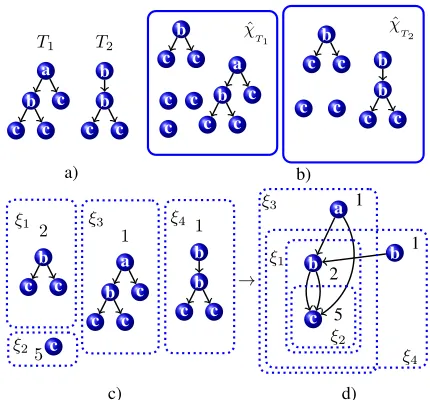
To compute the score for a model M the following is needed: the set of subtrees appearing in at least one tree in the model and, for each subtree, the correspondingfξ(M)
value. Fig. 1 reports an example of a model represented by two trees, T1 andT2 (Fig. 1-a), their decomposition into
subtrees (Fig. 1-b), and the corresponding set of subtrees and
fξ(M)values (Fig. 1-c). The recursive nature of the eq. (10)
implies the following inclusion relation between subtrees:
t1⊂t2ift1is identical to the subtree formed by a child node
oft2 and all of its descendants. As a consequence, if two
class representatives are in an inclusion relationship,ξ0⊂ξ00, then representing both two equivalence classes independently is redundant. Taking as an exampleξ00, what is needed is only the information that is not in common withξ0and then a reference toξ0for the information in common betweenξ0
andξ00. This is exemplified in Fig. 1: the equivalence class
ξ2is included inξ1,ξ1 ⊂ξ3, ξ1 ⊂ ξ4, ξ2 ⊂ξ3(Fig. 1-c);
for example the equivalence classξ3is represented by the
node labelled asa, together with its frequency1, and by links to the representatives of the classesξ1, ξ2(Fig. 1-d). Such
compact representation results in a forest of annotated DAGs.
7
Experiments
Semantic Role Labelling (SRL) is the task of automatically extracting a predicate along with its argument from a natural language sentence. Previous work has shown that Semantic
a
b
c c
c T1
b
b
c c
T2
a
b
c c
c b
c c
c c
c
ˆ χ
T1
b
b
c c
b
c c
c c
ˆ χ
T2
b
c c
2 ξ1
c 5 ξ2
a
b
c c
c 1 ξ3
b
b
c c
1 ξ4
a) b)
c)
→
a
b
c
b 1
1
2
5
d) ξ2 ξ1 ξ3
ξ4
Figure 1: a) a model formed by two trees,T1andT2; b) the
decomposition into parts of the two trees; c) the set of equiv-alence classes formed according to eq. (4); each classξis described by a representative subtree (ξχˆ), and the frequency
of the subtree in the model (fξ(M)); d) an inclusion
rela-tionship between subtrees is exploited to avoid redundancies when representing the same subtrees in different equivalence classes.
Role Labeling (SRL) can be carried out by applying machine learning techniques, e.g., (Gildea and Jurasfky 2002). The model proposed in (Moschitti 2004) applies tree kernels to subtrees enclosing the predicate/argument relation. More pre-cisely, each predicate and argument pair is associated with the minimal subtree that dominates the words contained in both pair members. For example, in Fig. 2, the subtrees in-side the three frames are the semantic/syntactic structures associated with the three arguments of the verbto bring, i.e.
SArg0,SArg1andSArgM.
Unfortunately, the large size of the PropBank corpus makes learning via tree kernels rather expensive in terms of execu-tion time, which becomes prohibitive when all the data is used. Consequently, the algorithms presented in the previous sections are very useful to speed up the learning/classification processes and make the kernel based approaches more appli-cable. The next section empirically shows the benefit of our DAG-based algorithms.
Space and Time Comparisons We measured the compu-tation time and the memory allocation (in terms of input tree nodes belonging to the model) for both the traditional Per-ceptron algorithm and the voted PerPer-ceptron based on DAGs. The target learning tasks were those involved in Semantic Role Labelling, specifically argument boundary detection, i.e., all the nodes of the sentence parse tree are classified in
refer-S
N
NP
D N
VP
V Mary
to brought
a cat PP
IN N
school Arg. 0
Arg. M Arg. 1
Predicate
NP
D N
VP
V
brought
a cat
SArg1 VP
V
to brought
PP
IN N
school S
N
V Mary
brought VP
SArg0 SArgM
Figure 2: Parse tree of the sentence ”Mary brought a cat to school” along with the PAF trees for Arg0, Arg1 and ArgM.
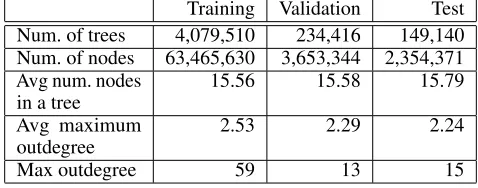
Training Validation Test Num. of trees 4,079,510 234,416 149,140 Num. of nodes 63,465,630 3,653,344 2,354,371 Avg num. nodes
in a tree
15.56 15.58 15.79
Avg maximum outdegree
2.53 2.29 2.24
Max outdegree 59 13 15
Table 1: Statistics of syntactic trees in the boundary detection dataset.
ring dataset, we used PropBank along with PennTree bank 2 (Marcus, Santorini, and Marcinkiewicz 1993). Specifically, we used all the sections of the PennTree bank for a total of 276,039 positive and 4,187,027 negative tree examples.
The DAG performance is affected by node distribution within trees along with their maximum and average out-degree. Table 1 reports statistics about the data derived from the boundary detection dataset. Note that there is a large number of relatively small trees, which can have a large out-degree. The total amount of nodes to be processed is almost 70 millions, thus, the dataset can demonstrate the computa-tional efficiency of our approach.
This dataset is almost prohibitive for computational expen-sive approaches such as SVM. It took 10,705 minutes just for processing 1 million examples with the faster SST ker-nel, e.g., about 7.5 days of computation. Thus we report the results obtained on the same experimental setting for the stan-dard and voted dag perceptrons. Fig. 3 shows the execution time for the standard perceptron and the voted dag percep-tron when using SST kernel combined with the polynomial kernel. In the case of the TKs and combination, we used the following parameters:λ∈ {0.2,0.3,0.4,0.5,0.6,0.7,0.8,
0.9,1.0}(TKs decay factor) andγ∈ {0.2,0.3,0.4,0.5,0.6,
0.7,0.8,0.9}(weighting the linear combination between tree and polynomial kernels). Only the values related to the faster and slower parameter settings are plotted.
Learning with the combination of kernels requires in the worst case (λ= 1.0andγ= 0.9)15,814.09seconds for the voted dag perceptron and22,892.62seconds for the standard perceptron in the most favorable case (λ= 0.6andγ= 0.9). Note that the voted perceptron, even in this unfavorable com-parison, is7078.53seconds faster (a bit less than2hours). Fig. 4 shows the memory usage of standard perceptron and
0 5000 10000 15000 20000 25000 30000
0 200000 400000 600000 800000 1e+06
Time in sec.
Number of tree examples Execution Time for Poly3 + Tk
Voted Dag Perceptron (λ=0.6 γ=0.7)
Voted Dag Perceptron (λ=1.0 γ=0.9)
Standard Perceptron (λ=0.6 γ=0.9)
Standard Perceptron (λ=1.0 γ=0.9)
Figure 3: Execution time in seconds for the Standard Percep-tron and the Voted DAG PercepPercep-tron over the training set with 1 million examples using a combination of Tk with different
λvalues and a polynomial kernel with degree 3 according to a parameterγ(Poly3+Tk). Only the slowest and fastest executions are reported.
voted dag perceptron algorithms.
The model created by the voted dag perceptron, when a combination of kernels is employed (Fig. 4), comprises from124,333to145,928nodes, while the model created by the standard perceptron comprises from391,240to625,501
nodes. The amount of nodes used by the standard perceptron can be more than4.2times higher than the one employed by the voted dag perceptron.
Finally, in Fig. 5 we report the training times for the voted dag perceptron on the full training set (i.e., up to 4,079,510 trees) when using the parameters selected on the validation set after training 1 million of tree examples. It can be noticed that the training is completed after129,163.98seconds (less than36hours) by using the polynomial kernel of degree 3,
51,235.9 seconds (a bit more than14hours) by using the SST kernel (λ= 0.4), and178,826.19seconds (less than50
0 50000 100000 150000 200000 250000 300000 350000 400000 450000 500000
0 200000 400000 600000 800000 1e+06
Number of nodes in memory
Number of tree examples Memory Usage for Poly3+Tk
Voted Dag Perceptron λ=0.4, γ=0.6 Voted Dag Perceptron λ=1.0, γ=0.6 Standard Perceptron λ=0.4, γ=0.4 Standard Perceptron λ=1.0, γ=0.6
Figure 4: Evolution of the number of tree nodes stored in memory and belonging to the model developed by the Stan-dard Perceptron and the Voted DAG Perceptron during train-ing on the traintrain-ing set with 1 million examples ustrain-ing the SST kernel combined with polynomial kernel. Only kernel parameters with largest and lower number of nodes stored are plotted.
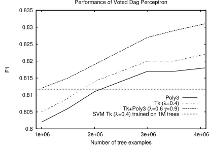
Accuracy Comparisons In Fig. 6 we report the accuracy measured by the F1, for the voted dag perceptron when using the kernels described above and the full training set. The figure also reports the F1 on the test set for SVM using the SST kernel (withλ= 0.4) and trained on the first million of tree examples. As expected, the voted (dag) perceptron us-ing the SST kernel trained on 1 million examples gets lower performance (0.805) than SVM. However, the performance steadily increases with the number of training examples. With 2 millions examples the voted perceptron gets a better accu-racy (0.814) in a much shorter training time, i.e., less than
4.3hours versus about7.5days of computation required for training SVM. When the full training set is used, the voted perceptron takes a bit more than14hours to learn a model able to reach an F1 of0.822, significantly improving the accu-racy over the SVM. Just using a degree 3 polynomial kernel for numerical features improves performance (up to0.818) as well (at the cost of a larger training time: see Fig. 5). The best performance is obtained by combining the two kernels: the training time still remains reasonable (on the full training set is less than50hours), while F1 increases up to0.831. In summary, the adoption of the dag-based approach allows to improve accuracy by using more examples at a fraction of the time needed by an SVM trained on 1 million examples.
8
Conclusions
In this paper, we have proposed a general approach to speed up the computation of the score function of classifiers based on kernel methods for structured data. Our methods avoid the re-computation of kernels over identical substructures appearing in different examples. We theoretically analyzed the formulation of the score, eq. (1), for Mapping Kernels, the most comprehensive framework for specifying kernel functions for structured data, and derived various strategies to find an optimal representation of the model: this allows
0 50000 100000 150000 200000
1e+06 2e+06 3e+06 4e+06
Time in sec.
Number of tree examples Execution Time for Voted Dag Perceptron
Poly3 Tk (λ=0.4) Tk+Poly3 (λ=0.6 γ=0.9)
Figure 5: Execution times of voted dag perceptron when using the full training set for polynomial kernel of degree 3 (Poly3), SST kernel (Tk), and a combination of the two (Tk+Poly3).
0.8 0.805 0.81 0.815 0.82 0.825 0.83 0.835
1e+06 2e+06 3e+06 4e+06
F1
Number of tree examples Performance of Voted Dag Perceptron
Poly3 Tk (λ=0.4) Tk+Poly3 (λ=0.6 γ=0.9) SVM Tk (λ=0.4) trained on 1M trees
Figure 6: Accuracy performance on the test set, as measured by the F1 measure, for polynomial kernel of degree 3 (Poly3), the SST kernel (Tk), a combination of the two (Tk+Poly3) and an SVM trained on 1 million examples using the SST kernel (SVM Tk).
to reduce its memory consumption and speed up the score computation. We showed that our findings apply to most pop-ular tree kernels. Finally, we provided empirical evidence of the benefit of our approach on Semantic Role Labelling task. We showed that the learning time of a perceptron algorithm on a large dataset of 4-million-instance decreases from more than a week to 14 hours only. It should be noted that our SVM-based model could only be trained on a significantly smaller number of examples. Thus, a simple voted percep-tron could outperform the SVM models also with respect to classification accuracy.
Acknowledgments
References
Aiolli, F.; Da San Martino, G.; Sperduti, A.; and Moschitti, A. 2007. Efficient Kernel-based Learning for Trees. InCIDM 2007, 308–315.
Anguita, D.; Ridella, S.; and Rivieccio, F. 2004. An algorithm for reducing the number of support vectors. InProceedings
of the WIRN04 XV Italian Workshop on Neural Networks.
Perugia, Italy.
Collins, M., and Duffy, N. 2002. New ranking algorithms for parsing and tagging: Kernels over discrete structures, and the voted perceptron. InACL02.
Crammer, K.; Dekel, O.; Keshet, J.; Shalev-shwartz, S.; and Singer, Y. 2006. Online Passive-Aggressive Algorithms.
Journal of Machine Learning Research7:551–585.
Cristianini, N., and Shawe-Taylor, J. 2000. An introduction to support vector machines and other kernel-based learning
methods. Cambridge University Press, 1 edition.
Croce, D.; Filice, S.; Castellucci, G.; and Basili, R. 2017. Deep Learning in Semantic Kernel Spaces. InACL’17
(Vol-ume 1: Long Papers), 345–354. Stroudsburg, PA, USA:
Association for Computational Linguistics.
Filice, S.; Da San Martino, G.; and Moschitti, A. 2015. Structural Representations for Learning Relations between Pairs of Texts. InProceedings of the 53rd Annual Meeting of the Association for Computational Linguistics (Volume 1:
Long Papers), 1003–1013. Beijing, China: Association for
Computational Linguistics.
Freund, Y., and Schapire, R. E. 1999. Large Margin Classifi-cation Using the Perceptron Algorithm.Machine Learning
37(3):277–296.
Gildea, D., and Jurasfky, D. 2002. Automatic labeling of semantic roles.Computational Linguistic28(3):496–530. Haussler, D. 1999. Convolution kernels on discrete struc-tures. Technical Report UCSC-CRL-99-10, University of California, Santa Cruz.
Jaakkola, T.; Diekhans, M.; and Haussler, D. 2000. A discrim-inative framework for detecting remote protein homologies.
Journal of Computational Biology7(1,2):95–114.
Kashima, H., and Koyanagi, T. 2002. Kernels for {Semi-Structured}Data. InProceedings of the Nineteenth
Interna-tional Conference on Machine Learning, 291–298. Morgan
Kaufmann Publishers Inc.
Kazama, J., and Torisawa, K. 2005. Speeding up training with tree kernels for node relation labeling. InHLT/EMNLP. Kazama, J., and Torisawa, K. 2006. Semantic role recog-nition using kernels on weighted marked ordered labeled trees. InProceedings of CoNLL-X, 53–60. New York City: Association for Computational Linguistics.
Kivinen, J.; Smola, A. J.; and Williamson, R. C. 2004. Online learning with kernels.Signal Processing, IEEE Transactions on52(8):2165–2176.
Kuang, R.; Ie, E.; Wang, K.; Wang, K.; Siddiqi, M.; Freund, Y.; and Leslie, C. S. 2004. Profile-based string kernels for remote homology detection and motif extraction. In
3rd International IEEE Computer Society Computational
Systems Bioinformatics Conference (CSB 2004), 152–160.
Marcus, M. P.; Santorini, B.; and Marcinkiewicz, M. A. 1993. Building a large annotated corpus of english: The Penn Tree-bank.Computational Linguistics19:313–330.
Moschitti, A., and Zanzotto, F. 2007. Fast and effective kernels for relational learning from texts. In Ghahramani, Z., ed.,Proceedings of the 24th Annual International Conference
on Machine Learning (ICML 2007), 649–656. Omnipress.
Moschitti, A. 2004. A study on convolution kernels for shallow semantic parsing. InProceedings of ACL’04. Moschitti, A. 2006. Efficient convolution kernels for de-pendency and constituent syntactic trees. In F¨urnkranz, J.; Scheffer, T.; and Spiliopoulou, M., eds.,ECML, volume 4212
ofLecture Notes in Computer Science, 318–329. Springer.
Nguyen, D., and Ho, T. 2006. A bottom-up method for simplifying support vector solutions. IEEE transactions on
neural networks17(3):792–796.
Rieck, K.; Krueger, T.; Brefeld, U.; and Mueller, K.-R. 2010. Approximate tree kernels. Journal of Machine Learning
Research11:555–580.
Rosemblatt, F. 1958. A probabilistic model for information storage and organization in the brain.Psychological Review
65:386–408.
Shawe-Taylor, J., and Cristianini, N. 2004. Kernel Methods
for Pattern Analysis. Cambridge University Press.
Shin, K., and Kuboyama, T. 2010. A Generalization of Haussler’ s Convolution Kernel — Mapping Kernel and Its Application to Tree Kernels. Journal of Computer Science
and Technology25(5):1040–1054.
Shin, K.; Cuturi, M.; and Kuboyama, T. 2011. Mapping kernels for trees. In Lise Getoor and Scheffer, T., ed., Pro-ceedings of ICML 2011, Bellevue, Washington, USA, June 28 - July 2, 2011, 961 – 968. Omnipress.
Shin, K. 2011. Mapping kernels defined over countably infinite mapping systems and their application. Journal of
Machine Learning Research20:367–382.
Tipping, M. E. 2001. Sparse bayesian learning and the relevance vector machine. Journal of Machine Learning
Research1:211–244.
Viswanathan, S., and Smola, A. J. 2003. Fast kernels for string and tree matching. In S. Becker, S. T., and Obermayer, K., eds.,NIPS 15. Cambridge, MA: MIT Press. 569–576. Wachsmuth, H.; Da San Martino, G.; Kiesel, D.; and Stein, B. 2017. The Impact of Modeling Overall Argumentation with Tree Kernels. InEMNLP 2017, 2369–2379. Copenhagen, Denmark: Association for Computational Linguistics. Zanzotto, F. M., and Moschitti, A. 2006. Automatic learning of textual entailments with cross-pair similarities. InACL. The Association for Computer Linguistics.